Potential Contribution of Residuals for Better Prediction of Soil
Salinity from Remote Sensing Data
Ahmed Eldiery1
Ph.D. Candidate, Civil Engineering Department, Colorado State University, Fort Collins CO 80523-1372.
Luis A. Garcia
Professor and Director, Integrated Decision Support Group, Civil Engineering Department, Colorado State University, Fort Collins CO 80523-1372.
Abstract. Soil salinity predictions derived from Ikonos and Landsat satellite images
are compared with field-collected soil salinity data for a study area in Colorado's lower Arkansas River Basin. The accuracy of the predictions is compared and issues of price, resolution, and coverage area are considered. Stepwise regression is used to select the combination of bands in the satellite images that best correlate with the field data. The Ordinary Least Squares (OLS) model is used to predict soil salinity using the combination of bands that resulted from the stepwise regression. The residuals for the OLS model are checked for whether they are roughly normal and approximately independently distributed with a mean of 0 and whether there is some constant vari-ance or not. If the residuals do not meet these conditions it means that there is some kind of autocorrelation among them. The SAR model is used to remove some of the autocorrelation among the residuals. If the SAR model does not give satisfactory re-sults, then a modified kriging model is used. The residuals of the OLS model which proved to have autocorrelation can be interpolated using kriging. The final predicted surface results from combining the surface produced from the OLS model with the surface produced by the kriged residuals. The results of this methodology to predict soil salinity from remote sensing data while taking into account the importance of re-siduals are promising.
1. Introduction
The development of saline soils is a dynamic phenomenon, which needs to be monitored regularly in order to secure up-to-date knowledge of their extent, spatial distribution, nature and magnitude (Ghassemi et al., 1995). Environ-mental damage occurs when saline water from drainage schemes or groundwa-ter is accumulated in off-stream floodplain areas or wetlands and either is left to evaporate naturally or discharged when high flow rates in the main stream prevail (Williams, 1987). When saline water is accumulated in floodplain areas or wetlands and left to evaporate, damage occurs directly in the areas inun-dated with saline water (Tanji et al., 1986).
The Arkansas River is one of the most saline rivers of its size in the United States. Salinity levels, measured as dissolved solid concentrations, increase from 300 mg/L near Pueblo to over 4,000 mg/L at the Colorado-Kansas border
1
Civil Engineering Department Colorado State University Fort Collins, CO 80523-1372 Tel: (970) 491-7620
(Ghassemi et al., 1995). Based on data collected over a 50,600 ha sub region of the Lower Arkansas Valley, Gates et al. (2002) stated that a shallow water ta-ble with an average salinity concentration of 3,100 mg/L spreads out under the land at an average depth of 2.1 m below the ground surface. Burkhalter et al (2005) mentioned that over three irrigation seasons, average seasonal aquifer recharge from irrigated fields in a 50,600 ha study area ranges from 0.59 to 0.99 m, including contribution from precipitation.
Remote sensing of surface features using aerial photography, videography, infrared thermometry and multispectral scanners has been used intensively to identify and map salt-affected areas (Robbins and Wiegand, 1990). Multispec-tral data acquired from platforms such as Landsat, SPOT, and the Indian Re-mote Sensing (IRS) series of satellites have been found to be useful in detect-ing, mapping and monitoring salt affected soils (Dwivedi and Rao, 1992). Sa-linity hazard mapping has included salt load studies, trend-based methodolo-gies, strongly inverse methods, composite index methods and integrated geo-science approaches (Lawrie et al., 2000, 2003; Spies and Woodgate, 2004). Composite index approaches have also more recently been further developed for salinity risk assessments (Clifton and Heislers, 2004). For mapping surface land salinity, color, and thermal infrared aerial photography and spectral image interpretation techniques such as satellite (Landsat TM, SPOT), and other air-borne remote sensing techniques are used (George et al., 2003; Spies and Woodgate, 2004). Other techniques, such as gamma radiometrics (Wilford et al., 2001), are useful for mapping soils and shallow sub-soil materials that can assist with interpretation of likely recharge and discharge areas.
The integration of remotely sensed data, Geographic Information Systems (GIS), and spatial statistics provides useful tools for modeling large-scale vari-ability to predict the distribution soil characteristics (Kalkhan and Stohlgren, 2000). Strong statistical tools for measuring autocorrelation available are Moran’s I (Moran 1948) and the spatial cross-correlation statistic (Bonham et al. 1995; Reich et al. 1994). Earlier research in the area of spatial statistics led to the development of a multivariate spatial correlation statistic by Wartenberg (1985) based on a mantle type coefficient to quantify the spatial relationships among univariate data (Reich et al., 1994). Goward et al. (1994) point out that while many spatial data sets describing land characteristics have proven reli-able for macro-scale ecological monitoring, these relatively coarse-scale data fall short in providing the precision required by more refined ecosystem re-source models.
2. Methods
In this study, the cross correlation between soil salinity data collected in the field with EM-38 probes and satellite imagery reflectance values is tested using a variety of techniques that include: ordinary least squares (OLS), the spatial autoregressive (SAR), and modified kriging models. Two images from the Ik-onos satellite one take on July 11, 2001 and another on July 1, 2004 and a Landsat image taken on July 8, 2001 are tested for cross correlation with soil salinity. In previous studies, individual tests of the best band or the best index
were conducted. In this study, a combination of all bands and vegetation index which proved to be good indicators of soil salinity based on vegetation are tested collectively and the ones that have the best cross correlation with soil sa-linity are selected.
To test for the cross correlation between the soil salinity data and the best combination of the satellite imagery, three different approaches are used and the residuals are examined for normality and spatial autocorrelation. The re-siduals indicate whether a chosen model is appropriate. The OLS model is fit for the soil salinity data and the combination of the image. If the residuals of the OLS model prove to have spatial autocorrelation, then SAR model is used. The same variables are then tested using the SAR model, which has the capa-bility of removing some of the spatial autocorrelation in the residuals. If the use of the SAR model does not give better results comparing the predicted val-ues versus the observed ones, then the modified kriging model is used. The modified kriging model involves kriging the residuals of the OLS model which proved to have spatial autocorrelation and combining the surfaces generated by the OLS model and the kriged residuals surface. The best model selected should provide the closest predicted data to the observed ones and no autocor-relation among the residuals.
3. Results and Analysis
3.1 Using the OLS model
The OLS model was tested using three sets of collected soil salinity data with the three acquired satellite images. The results of fitting the OLS model show strong correlation with the observed soil salinity data. The P-value of each separate band was less than 0.05. The mutable R2 shows values of 0.48, 0.52, 0.37 for the Landsat 2001, Ikonos 2001, and Ikonos 2004 images respec-tively. The AICC values were 1470, 959, and 1418 for the same images re-spectively. The Moran’s (I) P-values (2-side) were 0.49, 0.00, and 0.42 for the same images respectively. The Moran’s (I) P-value indicated that using the OLS model with the Landsat 2001 and Ikonos 2004 images might not be asso-ciated with autocorrelation among the residuals since the P-values are larger than 0.05. Yet the OLS model when used with the Ikonos 2001 image seems to produce autocorrelation among the residuals since the P-value is less than 0.05. In the meantime, the Lagrange P-value (2-side) was 0 for the three sets of data implying that there might be some spatial dependency or autocorrelation among the residuals. Therefore, there is a need to inspect the residuals graphi-cally for autocorrelation.
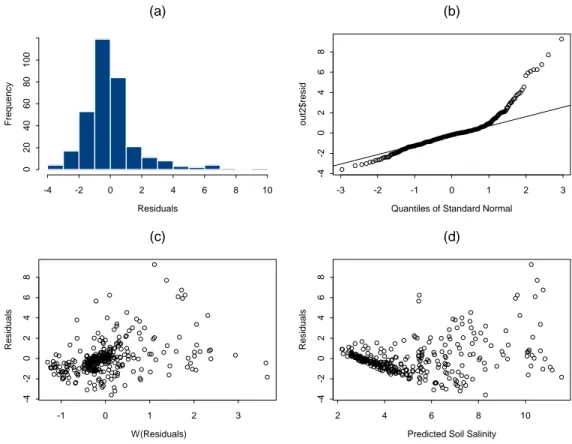
Figure 1 shows the residuals using the soil salinity data collected in 2001 in conjunction with the Landsat image. The two graphs at the top show the spection of the normality while the two graphs at the bottom display the in-spection of the homogeneity. The graph on the upper left shows the histogram of residuals. The histogram figure is not bell-shaped and is skewed to the left indicating that the distribution is not totally normal. The upper right graph (Q-Q) graphs the empirical quantiles based on residuals versus the corresponding
quantiles from a normal population. It is clear from the quantiles that all the points are very close to the line between the vales -3 to 1, and the points start to deviate from the line for the values above 1. This points to the fact that the distribution of the residuals is not totally normal. In the graph on the bottom left showing the residuals versus the weight of the residuals, there is some kind of pattern, no homogeneity, and some cluster in the distribution. The figure on the bottom right, the residuals versus the predicted values of soil salinity, shows that the distribution of points is not scattered randomly about 0. These results show that the residuals are dependently distributed, implying that there might be some spatial autocorrelation.
-5 0 5 10 0 2 0 4 0 6 0 8 0 120 Residuals Fr equenc y (a)
Quantiles of Standard Normal
out1$r es id -3 -2 -1 0 1 2 3 -5 0 5 1 0 (b) W(Residuals) Res iduals -2 0 2 4 6 -5 0 5 1 0 (c)
Predicted Soil Salinity
Res iduals 2 4 6 8 10 -5 0 5 1 0 (d)
Figure 1. Graphical inspection of the residuals of the OLS model.
3.2 Using the SAR model
The same data was tested again using the SAR model. The mutable R2 shows values of 0.18, 0.26, and 0.15 for the Landsat 2001, Ikonos 2001, and Ikonos 2004 images respectively. The AICC values were 1300, 888, and 1366 for the same images respectively. The likelihood ratio test P-value was 0 for the three data sets. The
λ
values were 0.98, 0.94, and 0.91 for the same im-ages respectively, which implies that there was significant autocorrelation among the residuals. The standard error ofλ
were 0.012, 0.032, and 0.04 for the same images respectively. Based on these numbers it is clear that the AICC values are better than those of the OLS and that there was some autocorrelation in the OLS model residuals. Figure 2 shows that the histogram of the variables with the SAR model is closer to a bell shape than that of the OLS model. Thismeans that the SAR model was able to make the distribution of residuals closer to normal. The quantiles figure behaves the same as that of the OLS model. The figure on the left, the residuals versus the weight of the residuals, shows no clear pattern and more homogeneity than that of the OLS model. These re-sults show that the residuals still have some dependency which means that there might be some spatial autocorrelation. Based on this analysis it is clear that the SAR model makes some contribution toward removing some autocor-relation among the residuals, but the R2 values are not encouraging. Therefore, the issue of the autocorrelation among the residuals needs to be dealt with in a better way. -4 -2 0 2 4 6 8 10 0 2 04 06 0 8 0 1 0 0 Residuals Frequency (a)
Quantiles of Standard Normal
out2$resid -3 -2 -1 0 1 2 3 -4 -2 024 68 (b) W(Residuals) Residuals -1 0 1 2 3 -4 -2 02 468 (c)
Predicted Soil Salinity
Residuals 2 4 6 8 10 -4 -2 02 468 (d)
Figure 2. Graphical inspection of the residuals using the OLS model.
3.3 Using the modified kriging model
The residuals of the OLS model proved to have spatial autocorrelation. Therefore, the residuals are kriged and combined with the OLS model. To ap-ply the kriging technique to the residuals, a best fit variogram was selected based on the smallest value of AICC. Having chosen the best variogram, the nearest neighbors number of the selected variogram should be selected based on the smallest variance.
Figure 3 shows the different variograms used in the kriging technique. Us-ing the Landsat 2001 image, the AICC values are 27.01, 21.74, and 15.03 for the Gaussian, spherical and exponential models respectively. For the same im-age, the standard errors were 2.07, 2.09, and 2.3. The AICC values for the Iko-nos 2001 image are 26.17, 24.69, and 23.98 for the Gaussian, spherical and
ex-ponential models respectively, and the standard errors were 1.55, 1.57, and 1.57. The AICC values for the Ikonos 2004 image are 48.90, 47.79, and 47.41 for the Gaussian, spherical and exponential models respectively. For the same image, the standard errors were 2.66, 2.66, and 2.75. It is clear from the figure that the exponential variogram fits the best of all the variograms. The exponen-tial model had the smallest AICC values. There was no significant difference among the standard error values of the three models.
xp yp 0 50 100 150 200 250 23 4 Exponential Spherical Gaussian
Fitting variogram models using all observed points from all fields
Comparison of the mean values of the OLS, the SAR, and the modified kriging models to the values of the collected soil salinity data
0.00 1.00 2.00 3.00 4.00 5.00 6.00 7.00
Field 17 Field 40 Field 80 All Fields
Field # Me an valu es OBS OLS SAR Modified Kriging
Figure 4. Comparison of the mean values of the OLS, the SAR, and the modified kriging
models to the values of the collected soil salinity data.
In addition to using the best variogram in the kriging technique, the best nearest neighbor number for the selected variogram (the exponential
variogram) needs to be decided based on the smallest variance. The nearest neighbors numbers used with the spherical variogram were 14, 12, and 10 for the Landsat 2001, Ikonos 2001, and Ikonos 2004 images respectively.
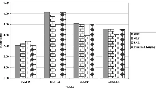
Figure 4 compares the means of the collected soil salinity data sets in the year 2001 with the predicted data using the Ikonos image and the OLS, SAR, and modified kriging models. For field 17, the mean value of the collected data was 3.02. The mean values were 3.25, 3.41, and 3.03 for the OLS, the SAR, and the modified kriging models respectively. For field 40, the mean value of the collected data was 6.13, while 5.86, 5.00, and 6.12 were the mean values of the OLS, the SAR, and the modified kriging models respectively. For field 80, the mean value of the collected data was 5.09 while 5.00, 3.95, and 5.04 were the mean values for the OLS, the SAR, and the modified kriging models re-spectively. For all the fields together, the mean of the collected data was 4.55. The mean values for the OLS, the SAR, and the modified kriging models were 4.53, 4.06, and 4.53 respectively. Figure 4 and the presented numbers show that the predicted soil salinity mean values produced by using the modifying kriging technique are very close to the mean values of the collected soil salin-ity data. Sometimes the OLS model comes closer than the modifying kriging model to predicting the soil salinity but not always. The SAR model is the least effective at predicting soil salinity.
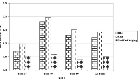
Figure 5 shows one example of comparing the absolute mean errors of the three different models when used to predict soil salinity from the Ikonos im-age. For field 17, the absolute mean error values were 0.70, 0.97, and 0.52, for the OLS, the SAR, and the modified kriging models respectively. For field 40,
Comparison of the absolute mean error values of the OLS, the SAR, and the modified kriging models
0.00 0.50 1.00 1.50 2.00 2.50
Field 17 Field 40 Field 80 All Fields
Field # M ean A b solut e Err o r OLS SAR Modified Kriging
Figure 5. Comparison of the absolute mean error values of the OLS, the SAR, and the
modified kriging models.
the absolute mean error values were 1.81, 1.96, and 0.58, for the OLS, the SAR, and the modified kriging models respectively. For field 80, the absolute mean error values were 1.31, 1.51, and 0.38, for the OLS, the SAR, and the modified kriging models respectively. For all fields together, the absolute mean error values were 1.21, 1.43, and 0.50, for the OLS, the SAR, and the modified kriging models respectively. Again, the above figure and the pre-sented numbers show that the absolute mean error values of using the modify-ing krigmodify-ing technique to predict soil salinity from the Ikonos image compared to the other models are the smallest. It is clear that the OLS model sometimes is second after the modifying kriging while the SAR model performs the worst. As in the previous figure, the best results were gained from considering the re-siduals. Also, selecting the best variogram based on the smallest AICC value and selecting the best nearest neighbors based on the smallest variance con-tributes some improvement to the predicted values using the modified kriging model.
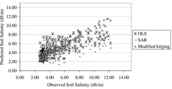
Figure 6 shows the predicted values using the three spatial models (OLS, SAR, and kriging models) versus the observed values of soil salinity when us-ing a Landsat image. It is obvious from this figure the there is a significant im-provement in R2 value when using kriged residuals combined with the OLS model over using the OLS or SAR models alone. The R2 values were 0.52 for the OLS model, 0.27 for the SAR model, and 0.82 for the modified kriging model. The modified kriging model produces predicted points with a clearer trend and more scatter than those of the OLS and the SAR models. In addition, the points tend to compose a line close to the 45 degree inclination which has an R2 value of 1. The other models deviate from this line.
The results of the other two sets of data show similar results. The data set
Comparison of predicted values of the OLS, the SAR, and the modified kriging models
0.00 2.00 4.00 6.00 8.00 10.00 12.00 14.00 0.00 2.00 4.00 6.00 8.00 10.00 12.00 14.00 Observed Soil Salinity (dS/m)
Predi cted Soil Salinit y (dS/m) OLS SAR Modified kriging `
Figure 6. Comparison of predicted values of the OLS, the SAR, and the modified kriging
models.
from 2001 combined with the Landsat image shows R2 values of 0.48, 0.40, and 0.80 for the OLS, the SAR, and the modified kriging models respectively. The 2004 data with the Ikonos image produces R2 values of 0.37, 0.15, and 0.76 for the OLS, the SAR, and the modified kriging models respectively.
Figure 7 shows the contribution of residuals when combined with the OLS model for field 7. The upper left figure (a) shows the kriged surface of the ob-served soil salinity. The upper right figure (b) shows the predicted surface of soil salinity resulting from the OLS model. The lower right figure (c) shows the kriged residuals of soil salinity resulting from the OLS model. The lower right figure (d) shows the final predicted surface of the soil salinity resulted from combining surfaces results from the OLS model and kriged residuals. It is clear from figure (b) that the OLS model behaves as a trend surface. The re-sulting surface shows the average of the points, but the high values are under-estimated and the low values are overunder-estimated. Kriging the residuals is able to fix the issue of underestimating and overestimating the high and low values as shown in figure (c). When surfaces (b) and (c) are combined to produce figure (d), the resulting predictions are very close to the observed salinity measure-ments.
Predicted soil salinity for Field 07 using Ikonos image for the year 2004 598600 598800599 000599200 599400599 600 X 421920 0 421 9400 421 9600 421980 0 4.2 2e6 422 0200 Y 0 5 1 0 1 5 2 0 Z a 598600598 800599000 599200599 400599600 X 421920 0 421 9400 421 9600 421 9800 4.2 2e6 422020 0 Y 4 6 8 1 0 Z b 598600598 800599000 599200599 400599600 X 421 9200 421 9400 421960 0 421 9800 4.22e6 422 0200 Y -5 0 5 1 0 Z c 598600598 800599000 599200599 400599600 X 421 9200 421 9400 421 9600 421 9800 4.22e6 422 0200 Y 0 5 1 0 1 5 2 0 Z d
Figure 7. Predicted soil salinity for Field 07 using Ikonos image for 2004
4. Conclusions
To generate high quality soil salinity maps, it is very important to chec the normality and spatial autocorrelation among residuals. In our research, the OLS model usually produced higher R2 values than the SAR model, but the OLS model was associated with autocorrelation in residuals. The SAR model was able to remove some of the autocorrelation in the residuals. When the re-siduals of the OLS model were kriged and combined with the OLS model, the results showed a significant improvement in R2 over the other models. On its own, the OLS model acts as a trend surface model; this means that it underes-timates the high values and overesunderes-timates the low values. The kriged residuals generate a surface that has positive and negative values which are added to the generated surface from the OLS model improving the predicted values by add-ing positive values to the underestimated values and addadd-ing negative values to the overestimated values. When using the modified kriging model, results are also improved by selecting the best variogram based on the smallest AICC value and selecting the best nearest neighbors based on the smallest variance.
References
Bonham, C.D., Reich, R.M., and Leader, K.K., 1995: A spatial cross-correlation of
Bouteloua gracilis with site factors. Grassland Science, 41, 196-201.
Burkhalter, J.P., and Gates, T.K., 2005: Agroecological impacts from salinization and waterlogging in an irrigated river valley. Journal of Irrigation and Drainage
En-gineering, ASCE, 131(2): In press.
Clifton,C.andHeislers,D.,2004: ASSALT: an asset based salinity priority setting approach. In 9th Murray-Darling Basin Groundwater Worskhop, 2004.
Dwivedi, R.S., and Rao, B.R.M., 1992: The selection of the best possible Landsat TM band combination for delineating salt-affected soils. International Journal of
Re-mote Sensing, 13 (11), 2051–2058.
Gates, T.K., Burkhalter, J.P., Labadie, J.W., Valliant, J.C., and Broner, I., 2002: Monitoring and modeling flow and salt transport in a salinity-threatened irrigated valley. Journal of Water Resources Planning and Management. 128(2), 87-99. George, R., Lawrie, K. C., and Woodgate, P., 2003: Convince me all your bloody
data and maps are going to help me manage salinity any better: A review of re-mote sensing methodologies for salinity mapping. 9th PURSL (Productive Use of Saline Land) Conference, Yepoon, Qld.
Ghassemi, F., Jackeman, A.J., and Nix, H.A., 1995: Salinization of land and water
re-sources : human causes, extent, management and case studies. CAB International,
Wallingford Oxon, UK.
Goward, S.N., Waring, R.H., Dye, D.G., and Yang, J.L., 1994: Ecological remote sensing at OTTER: Satellite macroscale observation. Ecological Applications, 4 (2), 322-343.
Kalkhan, M. A., and Stohlgren, T. J., 2000: Using multi-scale sampling and spatial cross-correlation to investigate patterns of plant species richness. Environmental
Monitoring and Assessment, 64 (3), 591-605.
Lawrie, K. C., Munday, T .J., Dent, D. L., Gibson, D. L., Brodie, R. C., Wilford, J., Reilly, N. S, Chan, R. A. and Baker, P., 2000: A ‘Geological Systems’ approach to understanding the processes involved in land and water salinisation in areas of complex regolith- the Gilmore Project, central-west NSW. AGSO Res. News., v. 32, p. 13-32, May 2000.
Lawrie, K. C., Please, P., and Coram, J., 2003: Groundwater quality (salinity) and distribution in Australia., 2003. In “Water, the Australian Dilemma”. Proceedings of the Annual Symposium of the Academy of Technological Sciences and Engi-neering, 17-18th Nov., Melbourne.
Lane, R., Brodie, R., and Fitzpatrick, A., 2004: Constrained inversion of AEM data from the Lower Balonne area, Southern Queensland, Australia. CRC LEME Open File Report 163.
Miles, D.L., 1977: Salinity in the Arkansas Valley of Colorado. U.S. Environmental Protection Agency, Interagency Agreement, Colorado State University, EPA-1AG-D4-0544, Fort Collins, CO.
Moran, P.A.P., 1948: The Interpretation of Statistical Maps, Roy. Stat. Soc., Ser. B. 10, 243-351.
Reich, R.M., Czaplewaki, R.L., and Bechthold, W.A., 1994: Spatial cross-correlation of undisturbed natural shortleaf pine stands in northern Georgia. Journal of
Envi-ronmental and Ecological Statistics, 1, 201-217.
Robbins, C.W., and Wiegand, C.L., 1990: Field and laboratory measurements.
Agri-cultural Salinity Assessment and Management, American Society of Civil
Spies, B. and Woodgate, P., 2004: Salinity mapping in the Australian context.
Tech-nical Report. Land & Water Australia.
Tanji, K., Läuchli, A., and Meyer, J., 1986: Selenium in the San Joaquin Valley.
En-vironment. 28(6), 6-11 and 34-39.
Wartenberg, D. 1985: Multivariable spatial correlation: a method for exploratory geographical analysis. Geographical Analysis, 17 (4), 263-283.
Wilford, J., R., Dent, D. L., Dowling, T. and Braaten, R., 2001: Rapid mapping of soils and salt stores using airborne radiometrics and digital elevation models.
AGSO Res. News., May 2001, p. 33-40.
Williams, W.D., 1987: Salinisation of rivers and streams: an important environmental hazard. Ambio, 16(4), 180-185.