Abstract—The Greater Zab and Lesser Zab are the major
tributaries of Tigris River contributing the largest flow volumes into the river. The impacts of climate change on water resources in these basins have not been well addressed. To gain a better understanding of the effects of climate change on water resources of the study area in near future (2049-2069) as well as in distant future (2080-2099), Soil and Water Assessment Tool (SWAT) was applied. The model was first calibrated for the period from 1979 to 2004 to test its suitability in describing the hydrological processes in the basins. The SWAT model showed a good performance in simulating streamflow. The calibrated model was then used to evaluate the impacts of climate change on water resources. Six general circulation models (GCMs) from phase five of the Coupled Model Intercomparison Project (CMIP5) under three Representative Concentration Pathways (RCPs) RCP 2.6, RCP 4.5, and RCP 8.5 for periods of 2049-2069 and 2080-2099 were used to project the climate change impacts on these basins. The results demonstrated a significant decline in water resources availability in the future.
Keywords—Tigris River, climate change, water resources,
SWAT.
I. INTRODUCTION
HE water resources of a basin are influenced by a large number of explanatory variables such as precipitation and other meteorological factors, vegetation and other landuse, and natural catastrophes such as hurricanes and bushfires. The water balance is often delicate, which can be easily exacerbated by climate change, especially when water resources are restricted [1]. Climate change can have a considerable impact on the hydrological cycles mainly through the modification of evapotranspiration and precipitation [2], [3]. The alterations of evapotranspiration and precipitation can, at the extreme, demonstrate formations of severe droughts or major floods leading to significant impacts on the water balance of a basin [4]. Greater Zab and Lesser Zab are the largest tributaries of Tigris River in terms of their contribution to Tigris flow. Greater Zab and Lesser Zab contribute about 40%-60% of total Tigris flow [5]. Furthermore, they are the main sources of surface water for Kurdistan region. Water scarcity has been pronounced in recent history in these basins [6]. Up till now, water problems in relation to climate change in the Greater Zab and Lesser Zab catchments have not been Nahlah Abbas and Saleh A Wasimi are with the school of engineering & technology, Central Queensland University, Melbourne, Australia (e-mail: n.abbas@cqu.edu.au, s.wasimi@cqu.edu.au).
Nadhir Al-Ansar is with Geotechnical Engineering, Lulea University of technology, 971 87 Lulea, Sweden (e-mail: nadhir.alansari@ltu.se).
well addressed [7]. Therefore, the main objective of this study has been to evaluate the potential impacts of future climatic changes in the water sources of these important basins, specifically blue and green waters. SWAT model was applied to determine the effects of climatic change on the watersheds. The model was set at monthly scale using available spatial and temporal data and calibrated against measured streamflow. Climate change scenarios were obtained from GCMs.
II. STUDY AREA
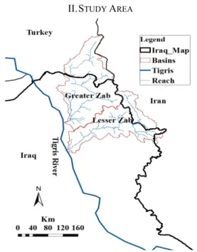
Fig. 1 Location of Greater Zab and Lesser Zab within Iraq
The Greater Zab rises from the Ararat Mountains in Turkey and flows through Turkey and the central northern part of Iraq and then joins the Tigris River south of Mosul City with a length of 372 km. The greater Zab is situated between latitudes 36 0N and 380N, and longitudes 43.3 0E and 44.3 0E [6] (Fig. 1). It drains an area of 26,473 km2, 65% of which is located in Iraq and the rest in Turkey [5]. Lesser Zab (also known as Little or Lower Zab) rises from north-eastern Zagros Mountains in Iran running through Iran and Iraq, and after a length of about 302 km, the river links with the Tigris River at Fatah (south of Mosul). The watershed is located approximately between 35.160N to 36.79 0N latitudes and its longitudes are 43.39 0E to 46.26 0E (Fig. 1). Lesser Zab serves an area of about 15,600 km2, 80% of which is located in Iraq and the remainder in Iran. The weather of the Greater Zab and
Nahlah Abbas, Saleh A. Wasimi, Nadhir Al-Ansari
Impacts of Climate Change on Water Resources of
Greater Zab and Lesser Zab Basins, Iraq, Using Soil
and Water Assessment Tool Model
T
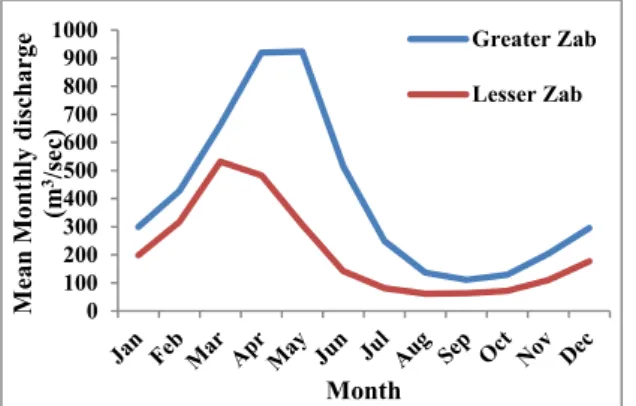
Lesser Zab watersheds is arid to semi-arid with dry and hot summers and wet winters [5]. The average annual temperature is variable from 22 °C in the south to 10 °C in the north. The average annual rainfall varies from 350 mm in the south and 1500 mm in the north [6].The flow regime of Greater Zab and Lesser Zab demonstrates high seasonal variability with peak flow occurring between April and May primarily due to snowmelt, and low seasonal flow occurring between July and December (Fig. 2). It is estimated that 70% of the catchment is covered by pasture and the rest is utilised for agriculture, Xerosols soil is the dominant in these basins [6].
Fig. 2 Average monthly streamflows of Greater Zab and Lesser Zab at EskiKelek and Dukan, respectively during 1979-2004
III. DESCRIPTION OF SWATMODEL
The SWAT model [8] is a river watershed, physics-based distributed model for analysing hydrology and water quality at different watershed scales with varying soils, land use and management conditions on a long-term basis. The model has two main divisions, land phase and routing phase, which apply to simulate the hydrology of a watershed. The land phase estimates the hydrological mechanisms which comprise evapotranspiration, surface runoff, subsurface water, ponds, lateral flow, channels and return flow [8]. The routing phase controls the movement of water, sediments, nutrients, and organic chemicals via the waterways network of the basin to the outlet [8].
In land phase of the hydrological cycle, the simulation is based on the water balance equation.
(1) where SWt (mm) is the final soil water content, SWo (mm) is the initial soil water content on day i, t(days) is the time, Rday
(mm) is the amount of precipitation on day i, Qsurf (mm) is the
amount of surface runoff on day i, Ea (mm) is the amount of
evapotranspiration on day i, Wseep (mm) is the amount of water entering the vadose zone from the soil profile on day i, and Qgw (mm) is the amount of return flow on day i. A
description of some of the major features of the model is shown in this study, and the full descriptions of the model can be provided in [9].
The estimation of surface runoff is conducted with two methods; the SCS curve number procedure [8] and the Green
and Ampt infiltration method [10]. The SCS method was applied in this study due to unavailability of sub-daily data that are essential for the Green and Ampt infiltration method.
The SCS curve number equation is: .
. (2) where, Qsurf (mm) is the accumulated runoff or rainfall excess,
Rday (mm) is the rainfall depth for the day, S(mm) is the
retention parameter.
The retention parameter diverges spatially owing to different soils, landuse, management and slope of a catchment and temporally because of soil water content variations. The retention parameter is defined by:
25.4 10 (3) where CN is the curve number for the day.
To estimate the retention component, SWAT 2012 utilizes the modified soil moisture method that permits the retention parameter to differ with plant evapotranspiration.
When the retention component is variable with soil profile water content, the equation below is applied,
∗ 1 ∗ (4)
where S (mm) is the retention parameter for a given day, Smax
(mm) is the maximum value that the retention parameter can achieve on any given day, SW(mm) is the soil water content of the entire profile excluding the amount of water held in the profile at wilting point, and w1 and w2 are shape coefficients.
The maximum retention parameter value, Smax (mm), is calculated by solving (3), using CN1, as shown below,
25.4 10 (5) In the case where the retention parameter is to be varied with plant evapotranspiration, the following equation is applied to calculate the retention parameter at the end of every day:
exp (6)
where Sprev (mm) is the retention parameter for the previous
day, Eo (mm/day) is the potential evapotranspiration for the
day, cncoef is the weighting factor used to estimate the retention coefficient for the daily curve number calculation which depends on plant evapotranspiration, Smax is the
maximum value of the retention parameter that can be achieved on any given day, Rday (mm) is the rainfall depth for the day, and Qsurf (mm) is the surface runoff. The initial value
of the retention parameter is defined as S = 0. 9Smax.
The model estimates the volume of lateral flow which depends on the variation in conductivity, slope and soil water
0 100 200 300 400 500 600 700 800 900 1000 M ean Month ly dis charge (m 3/s ec ) Month Greater Zab Lesser Zab
content. A kinematic storage model is used to predict lateral flow through each soil layer. Lateral flow is the flow below the soil surface when the water input into a layer exceeds the field capacity after percolation.
Regarding groundwater simulation, the process assumes two aquifers which are a shallow aquifer (unconfined) and a deep aquifer (confined) in each watershed. The shallow aquifer contributes streamflow into the main channel of the watershed.
The water balance equation for the shallow aquifer is:
, , . . (7)
where aqsh,i (mm) is the amount of water stored in the shallow
aquifer on day i, aqsh,i-1(mm) is the amount of water stored in
the shallow aquifer on day i-1, wrchrg.sh(mm) is the amount of
recharge entering the aquifer on day i, Qgw (mm) is the
groundwater flow, or base flow, into the main channel on day i, wrevap (mm) is the amount of water moving into the soil zone
in response to water deficiencies on day i, and wpump,sh (mm) is
the amount of water removed from the shallow aquifer by pumping on day i.
The steady-state response of groundwater flow to recharge is calculated by the equation given below [8].
∗ ∗
(8) where Ksat (mm/day) is the hydraulic conductivity of the
aquifer, Lgw (m) is the distance from the ridge or sub-basin
divide for the groundwater system to the main channel, and hwtbl (m) is the water table height.
Water infiltrating into the confined aquifer is presumed to contribute to the flow outside the watershed. SWAT model uses three methods to assess potential evapotranspiration (PET) – the Penman-Monteith method [11], the Priestley-Taylor method [12] and the Hargreaves method [13]. Water is directed via the streamflow network by using Muskingum river routing method utilizing the daily time step [8].
SWAT model demands an enormous amount of input data to achieve the tasks visualized in this research. Digital elevation model (DEM), landuse map, soil map, weather data and discharge data are basic data requirements for modelling. DEM was extracted from ASTER Global Digital Elevation Model (ASTERGDM) with a 30-meter grid and 1×1 degree tiles [14]. The land cover map was gathered from the European Environment Agency with a 250-meter grid raster for the year 2000 [15]. The soil map was obtained from the global soil map of the Food and Agriculture Organization of the United Nations (1995) [16]. Weather data which included daily precipitation, maximum and minimum temperatures were collected from the Iraq’s Bureau of Meteorology. Monthly streamflow data were obtained from the Iraqi Ministry of Water Resources/National Water Centre.
In SWAT model, the watershed is divided into smaller basins based on the DEM. The landuse map, soil map and slope datasets are embedded in the SWAT databases for this
study. The small basins are further sub-divided into Hydrologic Response Units (HRUs). HRUs are defined as parcels of land that have unique slope and soil and landuse area within the borders of a small basin. The HRUs represent percentages of sub-basin areas and hence are not spatially defined in the model. There must be at least one HRU in each small basin. HRUs enable the users to identify the differences in hydrologic conditions such as evapotranspiration for varied soils and landuses. Routing of water and pollutants is accomplished from the HRUs to the sub-basin level and then through the river system to the watershed outlet.
The Sequential Uncertainty Fitting Algorithm application (SUFI-2) is rooted in the SWAT-CUP model[17] was applied to assess the performance of the SWAT. The advantages of SUFI-2 are that it combines optimisation and uncertainty analysis, can handle large number of parameters through Latin hypercube sampling, and it is easy to apply. Moreover, SUFI-2 algorithm was found to achieve good prediction uncertainty with a limited number of runs comparing with other techniques connecting to SWAT such as generalized likelihood uncertainty (GLU) estimation, parameter solution (parsol), Markov Chain Monte Carlo (MCMC). This efficacy is of importance when the model is applying to complex and large basins [17].
Firstly, The SUFI-2 categorizes the dimension for each parameter. Thereafter, Latin Hypercube method is applied to produce different permutations among the calibration parameters. Finally, the model runs with each permutation, and the obtained results are compared with the observed data until the optimum objective function is reached. Because of the uncertainty in forcing inputs (e.g. temperature, rainfall), conceptual model and errors in measured data which are unavoidable in hydrological models, SUFI-2 algorithm computes the uncertainty of the measurements, the conceptual model and the parameters by two separate measures: P-factor and R-factor. P-factor is the percentage of data included by the 95% prediction uncertainty (PPU) which is bounded at 2.5% and 97.5% of the cumulative probability distribution of an output variable obtained from Latin Hypercube Sampling– it is similar to 95% confidence interval construction. The R-factor, which is standardized value, is the average width of the 95 PPU divided by the standard deviation of the corresponding measured variable. In an ideal scenario, P-factor tends towards 1 and R-factor towards zero. Furthermore, SUFI-2 calculates the Coefficient of Determination (R2) and the Nasch-Sutcliff efficiency (ENC) [18] to assess the goodness-of-fit between the measured and simulated data.
The ENC value indicates how well the plot of the observed against the simulated values fits the 1:1 line. It ranges from negative infinity (-∞) to one. The nearer the value to 1, the better is the prediction, while the value of less than 0.5 indicates unsatisfactory model performance [19]. ENC is calculated as shown below:
1 ∑∑ (9)
where Oi is the observed streamflow, Pi is the simulated
streamflow, and Ō is the mean observed streamflow during the evaluation period.
SUFI-2 allows users to accomplish global sensitivity analysis, which is computed based on the Latin Hypercube and multiple regression analysis. The multiple regression equation is defined as:
g α ∑ ∗
where g is the value of the evaluation index for the model simulations, α is a constant in the multiple linear regression equation, β is a coefficient of the regression equation, b is a parameter produced by the Latin hypercube method, and m is the number of parameters.
The t-stat of this equation which can indicate parameter sensitivity is applied to determine the relative significance of each parameter, the more sensitive the parameter, greater is the absolute value of the t-stat. When p-value is used, it is also an indication of the significance of the sensitivity, p-value close to zero has more significance.
Six GCMs from CMIP5 namely CGCM3.1/T47, CNRM-CM3, GFDL-CM2.1, IPSLCM4, MIROC3.2 (medres), and MRI CGCM2.3.2 were selected for climate change projections in the Lesser Zab basin under a very high emission scenario (RCP 8.5), a medium emission scenario (RCP 4.5) and a low emission scenario (RCP 2.6) for two future periods (2049-2069) and (2080-2099). Thereafter, the modelled temperatures and precipitation were input to the SWAT model and then water assets in the basin compare with the baseline period (1980-2010). BCSD method was applied to downscale the GCM results [20].
IV. RESULTS AND DISCUSSION A. Sensitivity Analysis
Sensitivity analysis was carried out for 25 parameters related to streamflow [8], from which 12 most sensitive parameters were considered for implementing in the model for calibration of the Greater Zab Basin. The rankings of 12 highest sensitive parameters for each watershed are presented in Table I. For Greater Zab, SFTMP was the greatest sensitive parameter. However, it was ranked the eighth for Lesser Zab. These results seem rational as Greater Zab river is snow-dominated mountainous terrain. CN2 was the dominant SWAT calibration parameter for Lesser Zab. However, it was ranked the fourth for Greater Zab. In a large number of SWAT applications in other watersheds, CN2 was the highest sensitive parameter [21]. CN2 tends to have the main impact on the quantity of runoff produced from the HRU, thus a relatively high sensitivity index can be expected for most of the basins [22]. SOL_AWC came third for Greater Zab and Lesser Zab. ALPHA-BE was observed to be the highest sensitive parameter among the four groundwater parameters for both watersheds. ALPHA-BE was ranked the second for Greater Zab and Lesser Zab. These results are similar to the findings of Li et al. [23] who found that ALPHA-BE is a
highly sensitive groundwater parameter in SWAT calibrations. SWAT was observed to be relatively sensitive to GW-DELY for Lesser Zab.
TABLEI
RANKS OF 12HIGHEST SENSITIVE PARAMETERS RELATED TO STREAMFLOW IN THE TWO BASINS IN IRAQ
Parameter Greater Zab Lesser Zab
CN2 4 1 ALPHA_BF 2 2 SFTMP 1 8 SOL_AWC 3 3 GW_DELAY 12 4 ESCO 8 11 HRU_SLP 5 7 SURLAG 7 5 GW_REVAP 11 6 GWQMN 9 9 SLSUBBSN 6 12 CH_K2 10 10
B. Calibration and Validation
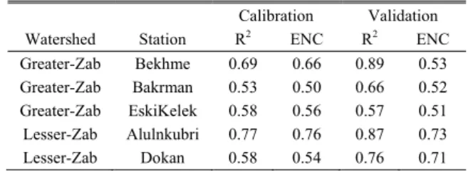
In both the basins, in spite of overestimates and underestimates during wet months, the model performed well over the whole simulation periods (Table II). The underestimation and overestimation during some months could be because of errors in measuring flow, unequally spread rainfall stations and spatial variability in soil and land use [24], [25]. Generally, the model can be assumed from the results to be capable of simulating the streamflow of the two basins.
TABLE II
R2 AND ENCVALUES IN THE BASINS
Calibration Validation Watershed Station R2 ENC R2 ENC
Greater-Zab Bekhme 0.69 0.66 0.89 0.53 Greater-Zab Bakrman 0.53 0.50 0.66 0.52 Greater-Zab EskiKelek 0.58 0.56 0.57 0.51 Lesser-Zab Alulnkubri 0.77 0.76 0.87 0.73 Lesser-Zab Dokan 0.58 0.54 0.76 0.71 C. Impacts of Climate Change on Tigris Basin Using CMIP5
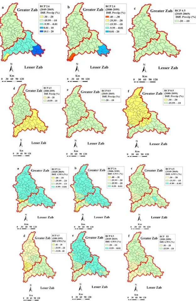
1) Precipitation Forecasts
Overall, all selected GCMs projected a reduction in the mean annual precipitation at about the mid-century (2049-2069) and about one-century lead time (2080-2099) for the two basins. Fig. 3 illustrates the anomaly maps of precipitation distribution (maps of percent deviation from historical data, (1980-2010) for RCP 2.6, RCP 4.5 and RCP 8.5 scenarios for the periods 2049-2069 and 2080-2099 for the average change from the multi-GCM ensemble. Under the RCP 2.6, Greater Zab is expected to experience a decrease of about 12% while the Lesser Zab 2% for the mid-century. At the end of the century, Greater Zab will experience nearly the same reduction, 15%, whereas Lesser Zab will experience a reduction of 10%. RCP 4.5 produced nearly the same reduction (average -18%) for both the basins in the
century, whereas at the end of the century, Greater Zab will see reduction of about -15%; however, the Lesser Zab will see 26% reduction. RCP 8.5 produced the same decreases for the half a-century in the two basins (17%), while for the end of the century, Greater Zab will experience a decline of about 22% and Lesser Zab 18%.
D. Blue Water and Green Water Forecasts
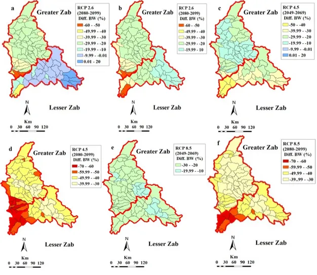
Fig. 4 captures the anomaly maps of blue water distribution (maps of percent deviation from historical data, 1980-2010) for RCP 2.6, RCP 4.5, and RCP 8.5 scenarios for the periods 2049-2069 and 2080-2099 from the average change of the multi-GCM ensemble. Under RCP 2.6, the half-a-century projection (2049-2069) shows a decline of about 29% and 22% in Greater Zab and Lesser Zab, respectively, while at the end of the century the reduction will be nearly the same in both the basins (27%). For RCP 4.5 (2049 -2069), Lesser Zab will see a decrease of about 33% followed by Greater Zab (20%). For RCP 4.5 (2080-2099), both the basins will experience approximately similar reduction of about 46%. Under RCP 8.5 both basins will experience a reduction of
about 23% for the period of (2049-2069). However, the Lesser Zab and Greater Zab will see a reduction of about 51% and 43%, respectively, for the period of (2080-2099). Green water has a tendency to have a similar trend as the blue water (Fig. 5).
Fig. 3 The impacts of climate change on the precipitation of the two basins (a) Anomaly based on scenario RCP 2.6 for the period 2049-2069, (b) Anomaly based on RCP 2.6 for 2080-2099, (c) Anomaly based on RCP 4.5 for 2049-2069, (d) Anomaly based on RCP 4.5 for 2080–2099, (e) Anomaly based on RCP 8.5 for 2049-264, and (f) Anomaly based on RCP 8.5 for 2080–2099.
Fig. 4 The impacts of climate change on the blue water of the two basins (a) Anomaly based on scenario RCP 2.6 for the period 2049-2069, (b) Anomaly based on RCP 2.6 for 2080-2099, (c) Anomaly based on RCP 4.5 for 2049-2069, (d) Anomaly based on RCP 4.5 for 2080–2099, (e) Anomaly based on RCP 8.5 for 2049-264, and (f) Anomaly based on RCP 8.5 for 2080–2099.
Fig. 5 The impacts of climate change on the green water of the two basins (a) Anomaly based on scenario RCP 2.6 for the period 2049-2069, (b) Anomaly based on RCP 2.6 for 2080-2099, (c) Anomaly based on RCP 4.5 for 2049-2069, (d) Anomaly based on RCP 4.5 for 2080–2099,
(e) Anomaly based on RCP 8.5 for 2049-264, and (f) Anomaly based on RCP 8.5 for 2080–2099
V. CONCLUSION
The findings from the SWAT model obviously reveal that the water system of the Greater Zab and Lesser Zab basins are likely to undergo alterations due to climate change, and most likely for the worse. The forecasts in the availability of water resources show declining trends. Since water is a limited resource for the region, a policy to deal with the adversity of the future is necessary. Certainly, preemptive intervention and pro-active actions would be highly beneficial and cost effective in the long term for the future generations.
REFERENCES
[1] H. Tabari, and P. Willems, 2016. Daily Precipitation Extremes in Iran: Decadal Anomalies and Possible Drivers. Journal of American Water Resources Association 52 (2): 541-599, DOI: 10.1111/1752-1688.12403.
[2] M. A. Mimikou, E. Baltas, E. Varanou, and K. Pantazis, 2000. Regional Impacts of Climate Change on Water Resources Quantity and Quality Indicators. Journal of Hydrology 234(1): 95-109, DOI:10.1016/S0022-1694(00)00244-4.
[3] J. M. Winter and E. A. B. Eltahir, 2012. Modeling the Hydroclimatology of the Midwestern United States. Part 1: Current Climate. Climate Dynamics 38(3-4): 573-593, DOI:10.1007/s00382-011-1182-2. [4] S. Selvanathan K. R. Sreetharan, D. Smirnov, J. Choi and M. Mampara,
2016. Developing Peak Discharges for Future Flood Risk Studies Using IPCC's CMIP5 Climate Model Results and USGS WREG Program. Journal of the American Water Resources Association 52 (4): 979-992, DOI: 10.1111/1752-1688.12407.
[5] UN-ESCWA and BGR, 2013. United Nations Economic and Social Commission for Western Asia; BundesanstaltfürGeowissenschaften und Rohstoffe. Inventory of Shared Water Resources in Western Asia. Beirut.
[6] N. Al-Ansari, S. Abdellatif, Ali and S. Knutsson, 2014. Long Term Effect of Climate Change on Rainfall in Northwest Iraq. Central European Journal of Engineering 4 (3): 250-263.
[7] I. E.Issa, N. Al-Ansari, G. Sherwany& S. Knutsson, Expected future of water resources within Tigris-Euphrates rivers basin, Iraq. Journal of Water Resource and Protection, 6, 2014, 421-432.
[8] J. G. Arnold, R. Srinivasan, R. S. Muttiah and J. R. Williams, 1998. Large Area Hydrologic Modeling and Assessment Part I: Model Development, Wiley Online Library.
[9] S. L. Neitsch, J. G Arnold, J. R Kiniry, R Williams and K. W King, 2005. Soil and water assessment tool theoretical documentation. Grassland. Soil and Water Research Laboratory, Temple, TX.
[10] W. H Green and G. A. Ampt, 1911. Studies on Soil Physics, Journal of Agricultural Science 4 (1): 1-24.
[11] J. L. Monteith, 1965. Evaporation and the Environment, in the State and Movement of Water in Living Organisms. Symposia of the Society of Experimental Biology 19:205-234.
[12] C. H. B. Priestley and R. J. Taylor, 1972. On the Assessment of Surface Heat Flux and Evaporation Using Large-Scale Parameters. Bulletin of American Meteorological Society 100(2): 81-92.
[13] G. L. Hargreaves, G. H. Hargreaves and J. P. Riley, 1985. Agricultural Benefits for Senegal River Basin. Journal of Irrigation and Drainage Engineering 111(2): 113-124.
[14] Jet Propulsion Laboratory California of Institute, 2012. Advanced Spacebome Thermal Emission and Reflection Radiometer, viewed 12, May 2015, https://asterweb.jpl.nasa.gov/gdem-wist.asp.
[15] European Environment Agency,2006, Spatial development of land use, viewed 23 May 2015, https://www.eea.europa.eu/data-and-maps. [16] Food and Agriculture Organization, 1995. The digital soil map of the
world and derived soil properties, Version 3.5, Rome
[17] K. C. Abbaspour, J. Yang, I. Maximov, R. Siber, K. Bogner, J. Mieleitner, J. Zobrist and R. Srinivasan, 2007. Modelling Hydrology and Water Quality in the Pre-Alpine/Alpine Thur Watershed Using SWAT. Journal of Hydrology 333(2-4): 413-430, DOI: 10.1016/j.jhydrol.2006.09.014.
[18] J. E. Nash and J.V. Sutcliffe, River flow forecasting through conceptual models part I—A discussion of principles. Journal of hydrology, 10(3), 1970, 282-290.
[19] D. N. Moriasi, J. G. Arnold, M. W. Van Liew, R. L. Bingner, R. D. Harmel and T. L Veith, 2007. Model evaluation guidelines for systematic quantification of accuracy in watershed simulations. Transactions of the ASABE 50(3): 885-900.
[20] E. P. Maurer, L. Brekke, T. Pruitt, B. Thrasher, J. Long, P. Duffy, M. Dettinger, D. Cayan& J. Arnold, An enhanced archive facilitating climate impacts and adaptation analysis. Bulletin of the American Meteorological Society, 95(7), 2014, 1011-1019.
[21] R. Cibin, K. P. Sudheer and I. Chaubey, Sensitivity and identifiability of stream flow generation parameters of the SWAT model. Hydrological processes, 24(9), 2010, 1133-1148.
[22] T. L. Veith, M. W. Van Liew, D. D. Bosch, and J. G. Arnold, 2010. Parameter Sensitivity and Uncertainty in SWAT: A Comparison across Five USDA-ARS Watersheds. Transactions of the ASABE 53 (5): 1477-1486.
[23] Z Li, Z. Xu, Q. Shao and J. Yang, 2009. Parameter Estimation and Uncertainty Analysis of SWAT Model in Upper Reaches of the Heihe River Basin. Hydrological Processes 23(19): 2744-2753.
[24] C. Santhi, J. G. Arnold, J. R. Williams, W. A. Dugas, R. Srinivasan and L. M. Hauck, 2001. Validation of the Swat Model on a Large Rwer Basin with Point and Nonpoint Sources1. Journal of the American Water Resources Association 37 (5):1169-1188.
[25] P. Ndomba, F. Mtalo and A. Killingtveit, 2008. SWAT Model Application in a Data Scarce Tropical Complex Catchment in Tanzania. Physics and Chemistry of the Earth Parts A/B/C 33 (8): 626-632.