Measurements of top quark spin observables in tt events using dilepton final states in root s=8 TeV pp collisions with the ATLAS detector

JHEP03(2017)113

Published for SISSA by Springer

Received: December 22, 2016 Revised: February 7, 2017 Accepted: March 1, 2017 Published: March 22, 2017

Measurements of top quark spin observables in t¯

t

events using dilepton final states in

√

s = 8 TeV pp

collisions with the ATLAS detector

The ATLAS collaboration

E-mail:

atlas.publications@cern.ch

Abstract: Measurements of top quark spin observables in t¯

t events are presented based on

20.2 fb

−1

of

√

s = 8 TeV proton-proton collisions recorded with the ATLAS detector at the

LHC. The analysis is performed in the dilepton final state, characterised by the presence

of two isolated leptons (electrons or muons). There are 15 observables, each sensitive to a

different coefficient of the spin density matrix of t¯

t production, which are measured

indepen-dently. Ten of these observables are measured for the first time. All of them are corrected

for detector resolution and acceptance effects back to the parton and stable-particle levels.

The measured values of the observables at parton level are compared to Standard Model

predictions at next-to-leading order in QCD. The corrected distributions at stable-particle

level are presented and the means of the distributions are compared to Monte Carlo

pre-dictions. No significant deviation from the Standard Model is observed for any observable.

Keywords: Hadron-Hadron scattering (experiments)

JHEP03(2017)113

Contents

1

Introduction

1

2

ATLAS detector

2

3

Observables

3

4

Data and simulation samples

5

5

Event selection and background estimation

7

5.1

Object selection

7

5.2

Event selection

8

5.3

Background estimation

8

5.4

Kinematic reconstruction of the t¯

t system

9

5.5

Event yields and kinematic distributions

9

6

Analysis

11

6.1

Truth level definitions

11

6.1.1

Parton-level definition

11

6.1.2

Stable-particle definition and fiducial region

12

6.2

Unfolding

13

6.3

Systematic uncertainties

14

6.3.1

Detector modelling uncertainties

17

6.3.2

Background-related uncertainties

18

6.3.3

Modelling uncertainties

18

6.3.4

Other uncertainties

19

7

Results

20

8

Conclusion

27

The ATLAS collaboration

33

1

Introduction

The top quark, discovered in 1995 by the CDF and D0 experiments at the Tevatron at

Fermilab [

1

,

2

], is the heaviest fundamental particle observed so far. Its mass is of the

order of the electroweak scale, which suggests that it might play a special role in

elec-troweak symmetry breaking. Furthermore, since the top quark has a very short lifetime

of O(10

−25

s) [

3

–

5

] it decays before hadronisation and before any consequent spin-flip can

JHEP03(2017)113

take place. This offers a unique opportunity to study the properties of a bare quark and,

in particular, the properties of its spin.

Top quarks at the LHC are mostly produced in t¯

t pairs via the strong interaction, which

conserves parity. The quarks

1

and gluons of the initial state are unpolarised, which means

that their spins are not preferentially aligned with any given direction. The top quarks

produced in pairs are thus unpolarised except for the contribution of weak corrections and

QCD absorptive parts at the per-mill level [

6

]. However, the spins of the top and antitop

quarks are correlated with a strength depending on the spin quantisation axis and on the

production process. Various new physics phenomena can alter the polarisation and spin

correlation due to alternative production mechanisms [

6

–

9

]. The spins of the top quarks do

not become decorrelated due to hadronisation, and so their spin information is transferred

to their decay products. This makes it possible to measure the top quark pair’s spin

structure using angular observables of their decay products. The predictions for many of

these observables are available at next-to-leading order (NLO) in quantum chromodynamics

(QCD). A few of them have been measured by the experiments at the LHC and Tevatron

and found to be in good agreement with the Standard Model (SM) predictions [

10

–

18

].

This paper presents the measurement of a set of 15 spin observables with a data set

corresponding to an integrated luminosity of 20.2 fb

−1

of proton-proton collisions at

√

s = 8

TeV, recorded by the ATLAS detector at the LHC in 2012. Each of the 15 observables

is sensitive to a different coefficient of the top quark pair’s spin density matrix, probing

different symmetries in the production mechanism [

19

]. Ten of these observables have not

been measured until now. The observables are corrected back to parton level in the full

phase-space and to stable-particle level in a fiducial phase-space. At parton level, the

measured values of the polarisation and spin correlation observables are presented and

compared to theoretical predictions. All observables allow a direct measurement of their

corresponding expectation value. At stable-particle level, the distributions corrected for

detector acceptance and resolution are provided. Because of the limited phase-space used

at that level, the values of the polarisation and spin correlations are not proportional to

the means of these distributions. Instead, the means of the distributions are provided and

compared to the values obtained in Monte Carlo simulation.

2

ATLAS detector

The ATLAS detector [

20

] at the LHC covers nearly the entire solid angle around the

interaction point.

2

It consists of an inner tracking detector surrounded by a thin

super-conducting solenoid, electromagnetic and hadronic calorimeters, and a muon spectrometer

incorporating superconducting toroid magnets.

1

Antiparticles are generally included in the discussions unless otherwise stated.

2

ATLAS uses a right-handed coordinate system with its origin at the nominal interaction point (IP) in the centre of the detector and the z-axis along the beam pipe. The x-axis points from the IP to the centre of the LHC ring, and the y-axis points upward. Cylindrical coordinates (r, φ) are used in the transverse plane, φ being the azimuthal angle around the beam pipe. The pseudorapidity is defined in terms of the polar angle θ as η = − ln[tan(θ/2)].

JHEP03(2017)113

The inner-detector system is immersed in a 2 T axial magnetic field and provides

charged-particle tracking in the pseudorapidity range |η| < 2.5. A high-granularity silicon

pixel detector covers the interaction region and typically provided three measurements per

track in 2012. It is surrounded by a silicon microstrip tracker designed to provide eight

two-dimensional measurement points per track. These silicon detectors are complemented by

a transition radiation tracker, which enables radially extended track reconstruction up to

|η| = 2.0. The transition radiation tracker also provides electron identification information

based on the fraction of hits (typically 30 in total) exceeding an energy-deposit threshold

consistent with transition radiation.

The calorimeter system covers the pseudorapidity range |η| < 4.9. Within the region

|η| < 3.2, electromagnetic calorimetry is provided by barrel and endcap high-granularity

lead/liquid-argon (LAr) electromagnetic calorimeters, with an additional thin LAr

pre-sampler covering |η| < 1.8 to correct for energy loss in the material upstream of the

calorimeters. Hadronic calorimetry is provided by a steel/scintillator-tile calorimeter,

seg-mented into three barrel structures within |η| < 1.7, and two copper/LAr hadronic endcap

calorimeters. The solid angle coverage is completed with forward copper/LAr and

tung-sten/LAr calorimeters used for electromagnetic and hadronic measurements, respectively.

The muon spectrometer comprises separate trigger and high-precision tracking

cham-bers measuring the deflection of muons in a magnetic field generated by superconducting

air-core toroids. The precision chamber system covers the region |η| < 2.7 with drift tube

chambers, complemented by cathode strip chambers. The muon trigger system covers the

range |η| < 1.05 with resistive plate chambers, and the range 1.05 < |η| < 2.4 with thin

gap chambers.

A three-level trigger system is used to select interesting events. The Level-1 trigger

is implemented in hardware and uses a subset of detector information to reduce the event

rate to a design value of at most 75 kHz. This is followed by two software-based trigger

levels, which together reduce the event rate to about 400 Hz.

3

Observables

The spin information of the top quarks, encoded in the spin density matrix, is transferred to

their decay particles and affects their angular distributions. The spin density matrix can be

expressed by a set of several coefficients: one spin-independent coefficient, which determines

the cross section and which is not measured here, three polarisation coefficients for the

top quark, three polarisation coefficients for the antitop quark, and nine spin correlation

coefficients. By measuring a set of 15 polarisation and spin correlation observables, the

coefficient functions of the squared matrix element can be probed. The approach used in

this paper was proposed in ref. [

19

]. The normalised double-differential cross section for t¯

t

production and decay is of the form [

6

,

21

]

1

σ

d

2

σ

d cos θ

a +

d cos θ

−b

=

1

4

(1 + B

a

JHEP03(2017)113

where B

a

, B

b

and C(a, b) are the polarisations and spin correlation along the spin

quanti-sation axes a and b. The angles θ

a

and θ

b

are defined as the angles between the momentum

direction of a top quark decay particle in its parent top quark’s rest frame and the axis a

or b. The subscript +(−) refers to the top (antitop) quark. From equation (

3.1

) one can

retrieve the following relation for the spin correlation between the axes a and b

C(a, b) = −9hcos θ

a₊

cos θ

−b

i.

(3.2)

Integrating out one of the angles in equation (

3.1

) gives the single-differential cross section

1

σ

dσ

d cos θ

a

=

1

2

(1 + B

a

_{cos θ}

a

_).

_(3.3)

This means the differential cross section has a linear dependence on the polarisation B

a

,

from which also follows

B

a

= 3hcos θ

a

i.

(3.4)

All the observables are based on cos θ, which is defined using three orthogonal spin

quantisation axes:

• The helicity axis is defined as the top quark direction in the t¯

t rest frame. In ref. [

19

] it

is indicated by the letter k, a notation which is adopted in this paper. Measurements

of the polarisation and spin correlation defined along this axis at 7 and 8 TeV were

consistent with the SM predictions [

10

–

16

].

• The transverse axis is defined to be transverse to the production plane [

6

,

22

] created

by the top quark direction and the beam axis. It is denoted by the letter n. The

polarisation along that axis was measured by the D0 experiment [

17

].

• The r-axis is an axis orthogonal to the other two axes, denoted by the letter r. No

observable related to this axis has been measured previously.

As the dominant initial state of t¯

t production at the LHC (gluon-gluon fusion) is

Bose-symmetric, cos θ calculations with respect to the transverse or r-axis are multiplied by the

sign of the scattering angle y = ˆ

p · ˆ

k, where ˆ

k is the top quark direction in the t¯

t rest

frame and ˆ

p = (0, 0, 1), as recommended in ref. [

19

]. In the calculations of cos θ with

respect to the negatively charged lepton, the axes are multiplied by −1. The observables

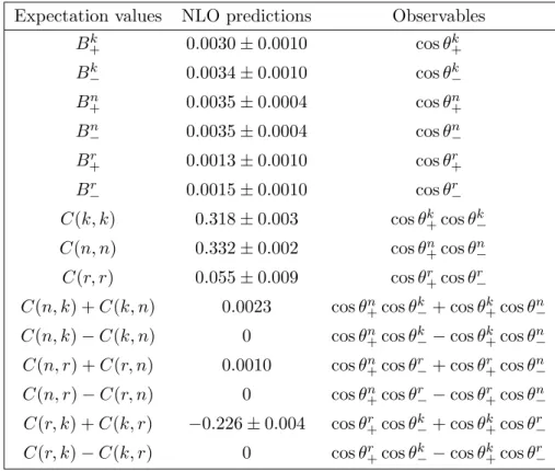
and corresponding expectation values, as well as their SM predictions at NLO, are shown

in table

1

. The first six observables correspond to the polarisations of the top and antitop

quarks along the various axes, the other nine to the spin correlations. In order to distinguish

between the correlation observables, the correlations using only one axis are referred to as

spin correlations and the last six as cross correlations. The predictions are computed for

a top quark mass of 173.34 GeV [

23

]. In order to measure all observables, the final-state

particles of both decay chains must be reconstructed and correctly identified. As charged

leptons retain more information about the spin state of the top quarks, and as they can be

precisely reconstructed, the measurement in this paper is performed in the dileptonic final

state of t¯

t events. The charged leptons considered in this analysis are electrons or muons,

either originating directly from W and Z decays, or through an intermediate τ decay.

JHEP03(2017)113

Expectation values

NLO predictions

Observables

B

₊k

0.0030 ± 0.0010

cos θ

₊k

B

−k

0.0034 ± 0.0010

cos θ

−k

B

₊n

0.0035 ± 0.0004

cos θ

₊n

B

₋n

0.0035 ± 0.0004

cos θ

₋n

B

₊r

0.0013 ± 0.0010

cos θ

₊r

B

−r

0.0015 ± 0.0010

cos θ

−r

C(k, k)

0.318 ± 0.003

cos θ

k₊

cos θ

₋k

C(n, n)

0.332 ± 0.002

cos θ

n₊

cos θ

−n

C(r, r)

0.055 ± 0.009

cos θ

r₊

cos θ

−r

C(n, k) + C(k, n)

0.0023

cos θ

n

+

cos θ

k−

+ cos θ

k+

cos θ

n−

C(n, k) − C(k, n)

0

cos θ

₊n

cos θ

k₋

− cos θ

k

+

cos θ

n−

C(n, r) + C(r, n)

0.0010

cos θ

₊n

cos θ

r−

+ cos θ

r+

cos θ

n−

C(n, r) − C(r, n)

0

cos θ

₊n

cos θ

r−

− cos θ

r+

cos θ

n−

C(r, k) + C(k, r)

−0.226 ± 0.004

cos θ

₊r

cos θ

k₋

+ cos θ

k₊

cos θ

r₋

C(r, k) − C(k, r)

0

cos θ

₊r

cos θ

k−

− cos θ

k+

cos θ

r−

Table 1. List of the observables and corresponding expectation values measured in this analysis. The SM predictions at NLO are also shown [19]; expectation values predicted to be 0 at NLO are exactly 0 due to term cancellations. The expectation values can be obtained from the corresponding observables using the relations from Equations (3.2) and (3.4). The uncertainties on the predictions refer to scale uncertainties only; values below 10−4 are not quoted.

4

Data and simulation samples

The analysis is performed using the full 2012 proton-proton collision data sample at

√

s = 8

TeV recorded by the ATLAS detector. The data sample corresponds to an integrated

luminosity of 20.2 fb

−1

after requiring stable LHC beams and a fully operational detector.

The analysis uses Monte Carlo (MC) simulations, in particular to estimate the sample

composition and to correct the measurement to both parton and stable-particle level. The

nominal t¯

t signal MC sample is generated by Powheg-hvq (version 1, r2330) [

24

–

27

] with

the top quark mass set to 172.5 GeV and the h

damp

parameter

3

set to the top quark

mass. The PDF set used is CT10 [

30

]. The signal events are then showered with Pythia6

(version 6.426) [

31

] using a set of tuned parameters named the Perugia2011C tune [

32

]. The

background processes are also modelled using a range of MC generators which are listed

in table

2

. An additional background originating from non-prompt and misreconstructed

(called “fake”) leptons is also estimated from MC simulation. To estimate this background,

all samples listed in table

2

are used, and in particular those listed in the lower part of

3_{The h}

damp parameter controls the hardness of the hardest emission which recoils against the t¯t

JHEP03(2017)113

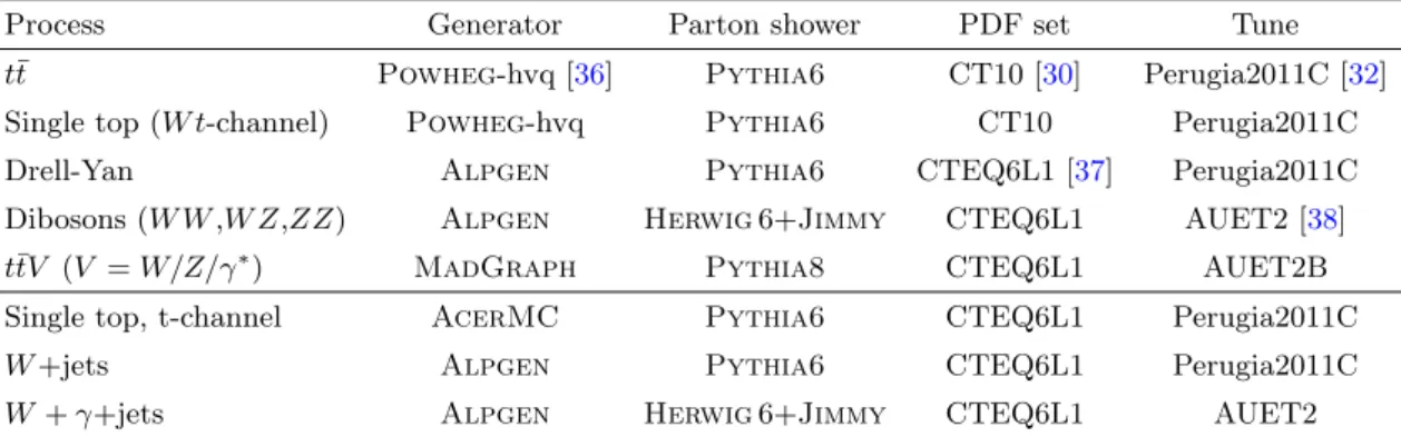
Process Generator Parton shower PDF set Tune

t¯t Powheg-hvq [36] Pythia6 CT10 [30] Perugia2011C [32]

Single top (W t-channel) Powheg-hvq Pythia6 CT10 Perugia2011C

Drell-Yan _{Alpgen Pythia6} CTEQ6L1 [37] Perugia2011C

Dibosons (W W ,W Z,ZZ) _{Alpgen Herwig 6+Jimmy} CTEQ6L1 AUET2 [38]

t¯tV (V = W/Z/γ∗) MadGraph Pythia8 CTEQ6L1 AUET2B

Single top, t-channel _{AcerMC Pythia6} CTEQ6L1 Perugia2011C

W +jets Alpgen Pythia6 CTEQ6L1 Perugia2011C

W + γ+jets Alpgen Herwig 6+Jimmy CTEQ6L1 AUET2

Table 2. MC generators and parton showers used for the signal and background processes. Samples in the lower part of the table are used together with the other samples to estimate the fake-lepton background. The parton distribution functions (PDF) used by the generator and the tunes used for the parton shower are also shown. The versions of the different generators are 2.14 for Alpgen [39], 5.1.4.8 for MadGraph [40_{], 4.31 for Herwig 6+Jimmy [}41_{], 1, r2330 for Powheg-hvq, 6.426 for}

Pythia6 [31] and 8.165 for Pythia8 [42].

Systematic uncertainty Generator Parton shower Tune Colour reconnection Powheg-hvq Pythia6

Perugia2012 [32] Perugia2012loCR Underlying event Powheg-hvq Pythia6

Perugia2012 Perugia2012mpiHi

Parton shower Powheg-hvq Pythia6

Perugia2011C

Herwig AUET2

Generator Powheg-hvq Herwig AUET2

MC@NLO

ISR/FSR Powheg-hvq Pythia6

Perugia2012radLo Perugia2012radHi

Top-quark mass _{Powheg-hvq Pythia6} Perugia2011C with various mass points

Table 3. List of t¯t samples used for studies of the modelling uncertainties. The PDF set is CT10 for all of them. The version of the MC@NLO generator [43,44] is 4.01.

the table, which are generated specifically for that background. Multijet events are not

included in this list because the probability of having two jets misidentified as isolated

leptons is very small. The contribution from these events is thus negligible.

In order to account for systematic uncertainties in the signal modelling, different MC

samples, documented in table

3

, are compared with each other as described in section

6.3.3

.

The nominal signal and background samples were processed through a simulation of

the detector geometry and response [

33

] using Geant4 [

34

]. MC samples used to estimate

signal modelling uncertainties were processed with the ATLFAST-II [

35

] simulation. This

employs a parameterisation of the response of the electromagnetic and hadronic

calorime-ters, and uses Geant4 for the other detector components.

JHEP03(2017)113

5

Event selection and background estimation

Reconstructed objects such as electrons, muons or jets are built from the detector

infor-mation and used to form a t¯

t-enriched sample by applying an event selection.

5.1

Object selection

Electron candidates are reconstructed by matching inner-detector tracks to clusters in the

electromagnetic calorimeter. A requirement on the pseudorapidity of the cluster |η

cl

| <

2.47 is applied, with the transition region between barrel and endcap corresponding to

1.37 < |η

cl

| < 1.52 excluded. A minimum requirement on the transverse momentum (p

T

)

of 25 GeV is applied to match the trigger criteria (see section

5.2

). Furthermore, electron

candidates are required to be isolated from additional activity in the detector. Two different

criteria are used. The first one considers the activity in the electromagnetic calorimeter in

a cone of size ∆R = 0.2 around the electron. The second one sums the p

T

of all tracks in a

cone of size 0.3 around the electron track. The requirements applied on both variables are

η-dependent and correspond to an efficiency on signal electrons of 90%. The final selection

efficiency for the electrons used in this analysis is between 85% and 90% depending on the

p

T

and η of the electron [

45

].

Muon candidates are reconstructed by combining inner detector tracks with tracks

constructed in the muon spectrometer. They are required to have a p

T

> 25 GeV and

|η| < 2.5. They are also required to be isolated from additional activity in the inner

detector. An isolation criterion requiring the scalar sum of track p

T

around the muon in

a cone of size ∆R = 10 GeV/p

µ_T

to be less than 0.05p

µ_T

is applied. Muons have a selection

efficiency of about 95% [

46

].

Jets are reconstructed from energy clusters in the electromagnetic and hadronic

calorimeters. The reconstruction algorithm used is the anti-k

t

[

47

] algorithm with a radius

parameter of R = 0.4. The measured energy of the jets is corrected to the hadronic scale

using p

T

- and η-dependent scale factors derived from simulation and validated in data [

48

].

After the energy correction, they are required to have a transverse momentum p

T

> 25

GeV and a pseudorapidity |η| < 2.5. For jets with p

T

< 50 GeV and |η| < 2.4, the jet vertex

fraction (JVF) must be greater than 0.5. The JVF is defined as the fraction of the scalar

p

T

sum of tracks associated with the jet and the primary vertex and the scalar p

T

sum

of tracks associated with the jet and any vertex. It distinguishes between jets originating

from the primary vertex and jets with a large contribution from other proton interactions

in the same bunch crossing (pile-up). If separated by ∆R < 0.2, the jet closest to a selected

electron is removed to avoid double-counting of electrons reconstructed as jets. Next, all

electrons and muons separated from a jet by ∆R < 0.4 are removed from the list of selected

leptons to reject semileptonic decays within a jet. Jets containing b-hadrons are identified

(b-tagged) by using a multivariate algorithm (MV1) [

49

] which uses information about the

tracks and secondary vertices. If the MV1 output for a jet is larger than a predefined value,

the jet is considered to be b-tagged. The value was chosen to achieve a b-tagging efficiency

of 70%. With this algorithm, the probability to select a light jet (from gluons or u-, d-,

s-quarks) is around 0.8%, and the probability to select a jet from a c-quark is 20%. The

JHEP03(2017)113

missing transverse momentum E

_Tmiss

is defined as the magnitude of the negative vectorial

sum of the transverse momenta of leptons, photons and jets, as well as energy deposits in

the calorimeter not associated with any physics object [

50

].

5.2

Event selection

The event selection aims at maximising the fraction of t¯

t events with a dileptonic final

state. The final states are then separated according to the lepton flavours. Tau leptons are

indirectly considered in the signal contribution when decaying leptonically. This leads to

three different channels (ee, µµ, eµ). Different kinematic requirements have to be applied

for the eµ and ee/µµ channels due to their different background contributions. Only events

selected from dedicated electron or muon triggers are considered. The p

T

thresholds of the

triggers are 24 GeV for isolated leptons and 60 (36) GeV for single-electron (-muon) triggers

without an isolation requirement. Events containing muons compatible with cosmic-ray

interactions are removed. Exactly two oppositely charged electrons or muons with p

T

> 25

GeV are required. A requirement on the dilepton invariant mass of m

``

> 15 GeV is required

in all channels. In addition, |m

``

−m

Z

| > 10 GeV, where m

Z

is the Z boson mass, is required

in the ee and µµ channels to suppress the Drell-Yan background. In these channels the

missing transverse momentum is required to be greater than 30 GeV. In the eµ channel, the

scalar sum of the p

T

of the jets and leptons in the event (H

T

) is required to be H

T

> 130

GeV. At least two jets with at least one of them being b-tagged are required in each channel.

5.3

Background estimation

Single-top-quark and diboson backgrounds are estimated using MC simulation only. The

MC estimate for the Drell-Yan and fake-lepton background is normalised using data-driven

scale factors (SF). The Drell-Yan background does not contain any real E

_Tmiss

.

Non-negligible E

_Tmiss

can appear in a fraction of events with misreconstructed objects, which

are difficult to model. Since real E

_Tmiss

is present in Z → τ τ events, no scale factors are

applied to this sample. Another issue is the correct normalisation of Drell-Yan events with

additional heavy-flavour (HF) jets from b- and c-quarks after the b-tagging requirement. In

order to correct for these effects, three control regions are defined, from which three SF are

extracted. Two correspond to the E

miss

T

modelling in Z → ee (SF

ee

) and Z → µµ events

(SF

µµ

), and one for the heavy-flavour normalisation in Z+jets events (SF

HF

) common to

the three dilepton channels. All control regions require the same selection as the signal

region with the exception that the invariant mass of the two leptons should be within

10 GeV of the Z mass. The control regions are then distinguished by dividing them into a

pretag (n

b-tag

≥ 0) and a b-tag region (n

b-tag

≥ 1), additionally dividing the pretag region

into the ee and µµ channels. The purity of the pretag control region is 97% on average for

both channels. The purity of the b-tag region is 75%. The SF are extracted by solving a

system of equations which relates the number of events in data and in simulation in the

three control regions. The lepton-flavour-dependent scale factors SF

ee/µµ

are 0.927 ± 0.005

and 0.890 ± 0.004 respectively for the ee and µµ channels while the heavy-flavour scale

factor SF

HF

is 1.70 ± 0.03, where the uncertainties are only statistical.

JHEP03(2017)113

The shape of the fake and non-prompt lepton background distributions are taken from

MC simulation but the normalisation is derived from data in a control region enriched in

fake leptons. This is achieved by applying the same requirements as for the signal region,

except that two leptons of the same charge are required. As fake leptons have approximately

the same probability of having negative or positive charge, the same number of fake-lepton

events should populate the opposite-sign and same-sign selection regions. The same-sign

control region has a smaller background contribution from other processes, allowing the

study of the modelling of the fake-lepton background. Channel-dependent scale factors are

derived by normalising the predictions to data in the control regions, while the shapes of

the distributions are taken from MC simulation. The SF in the ee and eµ channels are

around 1.0 and 1.5, whereas the SF in the µµ channel is about 4. The differences between

the three scale factors originate from the sources of misidentified electrons and muons,

which seem to be modelled better in MC simulation for the electrons. However, the shapes

of the distributions of several kinematic variables in the µµ channel are cross-checked in

control regions and found to be consistent with the distributions from a purely data-driven

method. The relative statistical uncertainties are about 20% in the same-flavour channels

and 10% in the eµ channel.

5.4

Kinematic reconstruction of the t¯

t system

The dileptonic t¯

t final state consists of two charged leptons, two neutrinos and at least two

jets originating from the top quark decay. As the neutrinos cannot be directly observed

in the detector, the kinematics of the t¯

t system, which is necessary to construct the

ob-servables, cannot be simply reconstructed from the measured information. To solve the

kinematic equations and reconstruct the t¯

t system, the neutrino weighting technique [

51

,

52

]

is used.

As input, the method uses the measured lepton and jet momenta. The masses of the

top quarks are set to their generated mass of 172.5 GeV whereas the masses of the W bosons

are set to their PDG values [

53

] in the calculations. A hypothesis is made for the value

of the pseudorapidity of each neutrino and the kinematics of the system is then solved.

For each solution found, a weight is assigned to quantify the level of agreement between

the vectorial sum of neutrino transverse momenta and the measured E

_Tmiss

components.

The pseudorapidities of the neutrinos are scanned independently between −5 and 5 with

fixed steps of 0.025 in the range [−2, 2] and of 0.05 outside of that range. All possible

combinations of jets and leptons are tested. Additionally, the resolution of the jet energy

measurement is taken into account by smearing the energy of each jet 50 times. The

smearing is done using transfer functions mapping the energy at particle level to the energy

after detector simulation. Out of all the solutions obtained, the one with the highest weight

is selected. The reconstruction efficiency of the kinematic reconstruction in the t¯

t signal

sample is about 88%. No solution is found for the remaining events.

5.5

Event yields and kinematic distributions

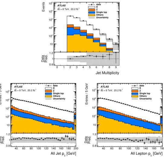
Figure

1

shows the jet multiplicity, lepton p

T

and jet p

T

for all three channels. Figure

2

recon-JHEP03(2017)113

Events 10 2 10 3 10 4 10 5 10 6 10 data t t Z Single top Others Uncertainty ATLAS -1 20.2 fb = 8 TeV, s Jet Multiplicity 0 1 2 3 4 5 6 7 8 9 Pred. Data 0.8 1 1.2 Entries / 5 GeV 10 2 10 3 10 4 10 5 10 data t t Z Single top Others Uncertainty ATLAS -1 20.2 fb = 8 TeV, s [GeV] T All Jet p 40 60 80 100 120 140 160 180 200 Pred. Data 0.8 1 1.2 Entries / 5 GeV 10 2 10 3 10 4 10 5 10 data t t Z Single top Others Uncertainty ATLAS -1 20.2 fb = 8 TeV, s [GeV] T All Lepton p 40 60 80 100 120 140 160 180 Pred. Data 0.8 1 1.2

Figure 1. Comparison of the number of jets, jet pTand lepton pTdistributions between data and

predictions after the event selection in the combined dilepton channel. The ratio between the data and prediction is also shown. The grey area shows the statistical and systematic uncertainty on the signal and background. The t¯tV , diboson and fake-lepton backgrounds are shown together in the “Others” category. Only the events passing the kinematic reconstruction are considered in the distributions.

struction. The data are well modelled by the MC predictions. The corrections to the

Drell-Yan and fake-lepton backgrounds are applied. Only the events passing the kinematic

reconstruction are considered in the distributions. The total number of predicted events is

slightly lower than the number of observed events, but the two are compatible within the

systematic uncertainties. The measurement is insensitive to a difference of normalisation

of the signal. There is also a slight slope in the ratio between data and prediction for the

lepton and top quark p

T

distributions. This is related to a known issue in the modelling

of the top quark p

T

, described in section

6.3.3

.

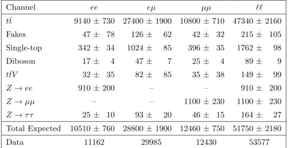
The final yields for each channel as well as for the inclusive channel combining ee, eµ

and µµ, along with their combined statistical and systematic uncertainties, can be found

in table

4

. The predictions agree with data within uncertainties in all channels.

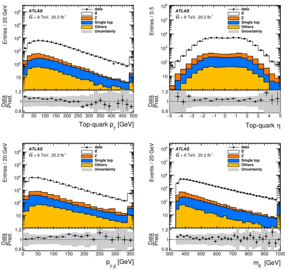
JHEP03(2017)113

Entries / 20 GeV 10 2 10 3 10 4 10 5 10 6 10 datatt Z Single top Others Uncertainty ATLAS -1 20.2 fb = 8 TeV, s [GeV] T Top-quark p 0 50 100 150 200 250 300 350 400 450 500 Pred. Data 0.8 1 1.2 Entries / 0.5 10 2 10 3 10 4 10 5 10 6 10 _data t t Z Single top Others Uncertainty ATLAS -1 20.2 fb = 8 TeV, s η Top-quark 5 − −4 −3 −2 −1 0 1 2 3 4 5 Pred. Data 0.8 1 1.2 Entries / 20 GeV 10 2 10 3 10 4 10 5 10 6 10 data t t Z Single top Others Uncertainty ATLAS -1 20.2 fb = 8 TeV, s [GeV] t T,t p 0 50 100 150 200 250 300 350 Pred. Data 0.8 1 1.2 Events / 20 GeV 10 2 10 3 10 4 10 5 10 6 10 datatt Z Single top Others Uncertainty ATLAS -1 20.2 fb = 8 TeV, s [GeV] t t m 300 400 500 600 700 800 900 1000 Pred. Data 0.8 1 1.2

Figure 2. Comparison between data and predictions after the kinematic reconstruction in the combined dilepton channel. The distributions of the top quark pTand η are shown, as well as the

t¯t pTand mass. The ratio between the data and prediction is also shown. The grey area shows the

statistical and systematic uncertainty on the signal and background. The t¯tV , diboson and fake-lepton backgrounds are shown together in the “Others” category. The last bin of the distribution corresponds to the overflow.

6

Analysis

Two different measurements of the spin observables are performed. One set of

measure-ments is corrected to parton level and the other set is corrected to stable-particle level.

These two levels are defined in the next section, as well as the phase-spaces to which the

measurements are corrected.

6.1

Truth level definitions

6.1.1

Parton-level definition

At parton level, the considered top quarks are taken from the MC history after radiation

but before decay. Parton-level leptons include tau leptons before they decay into an electron

JHEP03(2017)113

Channel

ee

eµ

µµ

``

t¯

t

9140 ± 730

27400 ± 1900

10800 ± 710

47340 ± 2160

Fakes

47 ± 78

126 ±

62

42 ± 32

215 ± 105

Single-top

342 ± 34

1024 ±

85

396 ± 35

1762 ±

98

Diboson

17 ±

4

47 ±

7

25 ±

4

89 ±

9

t¯

tV

32 ± 35

82 ±

85

35 ± 38

149 ±

99

Z → ee

910 ± 200

–

–

910 ± 200

Z → µµ

–

–

1100 ± 230

1100 ± 230

Z → τ τ

25 ± 10

93 ±

20

46 ± 15

164 ±

27

Total Expected

10510 ± 760

28800 ± 1900

12460 ± 750

51750 ± 2180

Data

11162

29985

12430

53577

Table 4. Event yields of t¯t signal, background processes and data after the full event selection and the kinematic reconstruction. The given uncertainties correspond to the combination of statistical and systematic uncertainties of the individual processes. The last column represents the inclusive dilepton channel.

or muon and before radiation. With these definitions, the polarisation can be extracted

from the slope of the cos θ distribution of parton-level particles (equation (

3.3

)) and the

correlation can be extracted from the mean value of the distribution (equation (

3.2

)). The

measurement corrected to parton level is extrapolated to the full phase-space, where all

generated dilepton events are considered.

6.1.2

Stable-particle definition and fiducial region

Stable-particle level includes only particles with a lifetime larger than 30 ps. The charged

leptons are required not to originate from hadrons. Photons within a cone of ∆R = 0.1

around the lepton direction are considered as bremsstrahlung and so their four-momenta

are added to the lepton four-momentum. Selected leptons are required to have p

T

> 25 GeV

and |η| < 2.5. Jets are clustered from all stable particles, excluding the already selected

leptons, by an anti-k

t

algorithm with a radius parameter R = 0.4. Neutrinos can be

clustered within jets. Intermediate b-hadrons have their momentum set to zero, and are

allowed to be clustered into the jets along with the stable particles [

54

]. If after clustering a

b-hadron is found in a jet, the jet is considered as b-tagged [

54

]. Jets must have a transverse

momentum of at least 25 GeV and have a pseudorapidity of |η| < 2.5. Events are rejected if

a lepton and a jet are separated by ∆R < 0.4. A fiducial phase-space close to the detector

and selection acceptance is defined by requiring the presence of at least two leptons and

at least two jets satisfying the kinematic selection criteria. Around 32% of all generated

events satisfy the fiducial requirements. No b-jet is required in the definition of the fiducial

region to keep it common with other analyses not using b-tagging. The b-jets are used in

the kinematic reconstruction described in the following.

JHEP03(2017)113

The top quarks (called pseudo-top-quarks [

55

]) are reconstructed from the stable

par-ticles defined above. If no jets are b-tagged, the two highest-p

T

jets are considered for the

pseudo-top-quark reconstruction. Neutrinos are required not to originate from hadrons,

but from W or Z decays or from intermediate tau decays. For the reconstruction, only the

two neutrinos with the highest p

T

are taken in MC events. The correct lepton-neutrino

pairings are chosen as those with reconstructed masses closer to the W boson mass. The

correct jet-lepton-neutrino pairings are then chosen as those with masses closer to the

generated top quark mass of 172.5 GeV.

In contrast to the parton-level measurement where all events are included, events from

outside the fiducial region can still pass the event selection at reconstruction level and have

to be treated as additional background (called the non-fiducial background). This

contri-bution is estimated from background-subtracted data by applying the binwise ratio of

non-fiducial to total reconstructed signal events obtained from MC simulation, which is found to

be constant for different levels of polarisation and correlation with an average of about 6.5%.

6.2

Unfolding

Selection requirements and detector resolution distort the reconstructed distributions. An

unfolding procedure is applied to correct for these distortions. The Fully Bayesian

Unfold-ing [

56

] method is used. It is based on Bayes’ theorem and estimates the probability (p) of

T ∈ R

Nt

_{being the true spectrum given the observed data D ∈ N}

Nr

_.

4

_{This probability is}

proportional to the likelihood (L) of obtaining the data distribution given a true spectrum

and a response matrix M ∈ R

Nr

_{× R}

Nt

_{. This can be expressed as}

p (T |D, M) ∝ L (D|T , M) · π (T ) ,

(6.1)

where π is the prior probability density for the true spectrum T and is taken to be uniform.

The background is estimated as described in section

5.3

and included in the computation

of the likelihood by taking into account its contribution in data when comparing it with

the true spectrum. The response matrix M, in which each entry M

ij

gives the probability

of an event generated in bin i to be reconstructed in bin j, is calculated from the nominal

signal sample. By taking a rectangular response matrix connecting the three different

anal-ysis channels to the same true spectrum, the channels are combined within the unfolding

method. The unfolded value is taken to be the mean of the posterior distribution with its

root mean square taken as the uncertainty.

Different systematic uncertainties are estimated within the unfolding by adding

nui-sance parameter terms (θ) to the likelihood for each systematic uncertainty considered.

The so-called marginal likelihood is then defined as

L (D|T ) =

Z

L (D|T , θ) · π(θ)dθ,

(6.2)

where π(θ) is the prior probability density for each nuisance parameter θ. They are

de-fined as Gaussian distributions G with a mean of zero and a width of one. Systematic

4

R and N are the sets of real and natural numbers. Nt and Nr are the number of bins for the true and

JHEP03(2017)113

uncertainties can be distinguished between normalisation-changing uncertainties (θ

n

) and

uncertainties changing both the normalisation and the shape (θ

s

) of the reconstructed

dis-tribution of signal R(T ; θ

s

) and background B(θ

s

, θ

n

). The marginal likelihood can then

be expressed as:

L (D|T ) =

Z

L (D|R(T ; θ

s

), B(θ

s

, θ

b

)) · G(θ

s

) · G(θ

b

)dθ

s

dθ

b

.

(6.3)

The method is validated by performing a linearity test in which distributions with

known values of the polarisation and spin correlations are unfolded. The distributions

of observables are reweighted to inject different values of the polarisations and

correla-tions.

For the polarisations and spin correlations, the double-differential cross section

(equation (

3.1

)) is used, while a linear reweighting is used for the cross correlations. The

unfolded value for each reweighted distribution is then compared to the true value of

po-larisation or spin correlation and a calibration curve is built. Non-closure in the linearity

test appears as a slope different from one in the calibration curve. The number of bins

and the bin widths for each observable are chosen based on its resolution and optimised by

evaluating the expected statistical uncertainty and by limiting the bias in the linearity test.

The binning optimisation leads to a four-bin configuration for the polarisation observables

and six-bin configurations for the different correlation observables. An uncertainty is added

to cover the non-closure of the linearity test, which is at most 10%. The input distribution

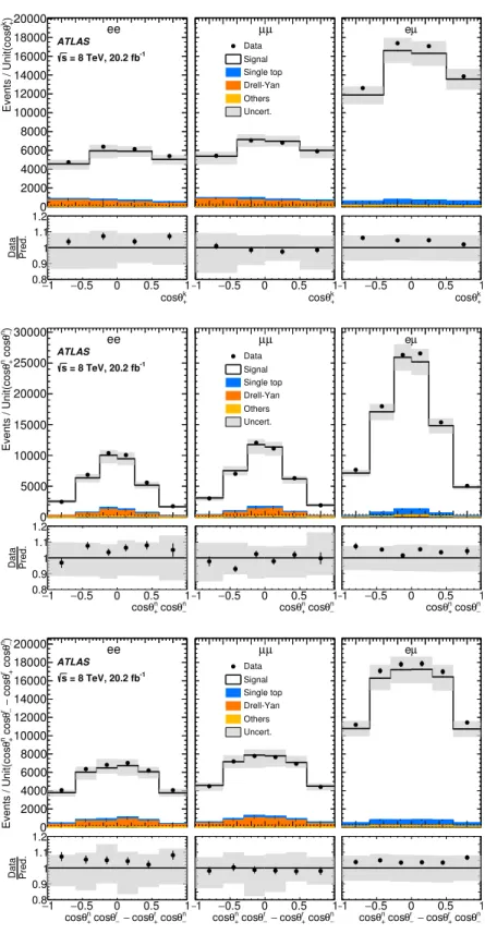
and the response matrix normalised per true bin are shown for one example of polarisation,

spin correlation, and cross correlation in figures

3

and

4

.

6.3

Systematic uncertainties

The measurement of the spin observables is affected in various ways by systematic

uncer-tainties. Three different types of systematic uncertainties are considered: detector

mod-elling uncertainties affecting both the signal and background, normalisation uncertainties of

the background, and modelling uncertainties of the signal. The first two types are included

in the marginalisation procedure. The reconstructed distribution, varied to reflect a

system-atic uncertainty, is compared to the nominal distribution and the average change per bin is

taken as the width of the Gaussian prior, as discussed in section

6.2

. In order to estimate the

impact of each source of systematic uncertainty individually, pseudodata corresponding to

the sum of the nominal signal and background samples are used. The unfolding procedure

with marginalisation is applied to the pseudodata and constraints on the systematic

uncer-tainties are obtained. The strongest constraint is on the uncertainty related to the electron

identification and it reduces this systematic uncertainty by 50%. The other constraints

are of the order of a few percent. The constrained systematic uncertainties are then used

to build the ±1σ variations of the prediction. The varied pseudodata are then unfolded

without marginalisation. The impact of each systematic uncertainty is computed by taking

half of the difference between the results obtained from the ±1σ variations of pseudodata.

Modelling systematic uncertainties for the signal process are estimated separately by

building calibration curves for each sample. The unfolded value in data is calibrated to

generator level using the calibration curves for the nominal sample and the sample varied

to reflect the uncertainty. The difference is taken as the systematic uncertainty.

JHEP03(2017)113

) k +_θ Events / Unit(cos 0 2000 4000 6000 8000 10000 12000 14000 16000 18000 20000 ATLAS -1 = 8 TeV, 20.2 fb s ee Data Signal Single top Drell-Yan Others Uncert. µ µ eµ k + θ cos 1 − −0.5 0 0.5 1 Pred. Data 0.8 0.9 1 1.1 1.2 k + θ cos 1 − −0.5 0 0.5 1 k + θ cos 1 − −0.5 0 0.5 1 ) n_θ− cos n_θ+ Events / Unit(cos 0 5000 10000 15000 20000 25000 30000 ATLAS -1 = 8 TeV, 20.2 fb s ee Data Signal Single top Drell-Yan Others Uncert. µ µ eµ n − θ cos n + θ cos 1 − −0.5 0 0.5 1 Pred. Data 0.8 0.9 1 1.1 1.2 n − θ cos n + θ cos 1 − −0.5 0 0.5 1 n − θ cos n + θ cos 1 − −0.5 0 0.5 1 ) n − θ cos r_θ+ cos − r − θ cos n + θ Events / Unit(cos 0 2000 4000 6000 8000 10000 12000 14000 16000 18000 20000 ATLAS -1 = 8 TeV, 20.2 fb s ee Data Signal Single top Drell-Yan Others Uncert. µ µ eµ n − θ cos r + θ cos − r − θ cos n + θ cos 1 − −0.5 0 0.5 1 Pred. Data 0.8 0.9 1 1.1 1.2 n − θ cos r + θ cos − r − θ cos n + θ cos 1 − −0.5 0 0.5 1 n − θ cos r + θ cos − r − θ cos n + θ cos 1 − −0.5 0 0.5 1

Figure 3. Input distributions for the unfolding procedure of cos θk

+, cos θn+cos θn−, and

cos θn

+cos θ−r − cos θ+r cos θ−n. The ratio between the data and prediction is also shown. The grey

area shows the total uncertainty on the signal and background. The t¯tV , diboson and fake-lepton backgrounds are shown together in the “Others” category.

JHEP03(2017)113

Figure 4. Response matrices of observables cos θk

+, cos θn+cos θn−, and cos θn+cos θr−− cos θr+cos θn−.

at parton level. They are divided into ee, µµ, and eµ channels. The matrices are normalised per truth bin (rows) for each channel separately.

JHEP03(2017)113

6.3.1

Detector modelling uncertainties

All sources of detector modelling uncertainty are discussed below.

Lepton-related uncertainties.

• Reconstruction, identification and trigger. The reconstruction and

identifi-cation efficiencies for electrons and muons, as well as the efficiency of the triggers

used to record the events differ between data and simulation. Scale factors and their

uncertainties are derived using tag-and-probe techniques on Z → `

+

`

−

(` = e or µ)

events in data and in simulated samples to correct the simulation for these

differ-ences [

57

,

58

].

• Momentum scale and resolution. The accuracy of the lepton momentum scale

and resolution in simulation is checked using the Z → `

+

`

−

and J/Ψ → `

+

`

−

invari-ant mass distributions. In the case of electrons, E/p studies using W → eν events are

also used. Small differences are observed between data and simulation. Corrections

to the lepton energy scale and resolution, and their related uncertainties are also

considered [

57

,

58

].

Jet-related uncertainties.

• Reconstruction efficiency. The jet reconstruction efficiency is found to be about

0.2% lower in the simulation than in data for jets below 30 GeV and it is consistent

with data for higher jet p

T

.

To evaluate the systematic uncertainty due to this

small inefficiency, 0.2% of the jets with p

T

below 30 GeV are removed randomly and

all jet-related kinematic variables (including the missing transverse momentum) are

recomputed. The event selection is repeated using the modified number of jets.

• Vertex fraction efficiency. The per-jet efficiency to satisfy the jet vertex fraction

requirement is measured in Z → `

+

`

−

+ 1-jet events in data and simulation,

select-ing separately events enriched in hard-scatter jets and events enriched in jets from

pile-up. The corresponding uncertainty is estimated by changing the nominal JVF

requirement value and repeating the analysis using the modified value.

• Energy scale. The jet energy scale (JES) and its uncertainty were derived by

combining information from test-beam data, LHC collision data and simulation [

48

].

The jet energy scale uncertainty is split into 22 uncorrelated sources, which have

different jet p

T

and η dependencies and are treated independently.

• Energy resolution. The jet energy resolution was measured separately for data

and simulation. A systematic uncertainty is defined as the difference in quadrature

between the jet energy resolutions for data and simulation. To estimate the

cor-responding systematic uncertainty, the jet energy in simulation is smeared by this

residual difference.

• b-tagging/mistag efficiency. Efficiencies to tag jets from b- and c-quarks in the

simulation are corrected by p

T

- and η-dependent data/MC scale factors. The

uncer-tainties on these scale factors are about 2% for the efficiency for b-jets, between 8%

and 15% for c-jets, and between 15% and 43% for light jets [

59

,

60

].

JHEP03(2017)113

The dominant uncertainties in this category are related to lepton reconstruction,

iden-tification and trigger, jet energy scale and jet energy resolution. The contribution from

this category to the total uncertainty is small (less than 20% for all observables).

Missing transverse momentum.

The systematic uncertainties associated with the

momenta and energies of reconstructed objects (leptons and jets) are propagated to the

E

_Tmiss

calculation. The E

_Tmiss

reconstruction also receives contributions from the presence

of low-p

T

jets and calorimeter energy deposits not included in reconstructed objects (the

“soft term”). The systematic uncertainty associated with the soft term is estimated using

Z → µ

+

µ

−

events using methods similar to those used in ref. [

61

]. The effect of this

procedure on the measured observables is minor.

6.3.2

Background-related uncertainties

The uncertainties on the single-top-quark, t¯

tV , and diboson backgrounds are 6.8%, 10%,

and 5%, respectively [

62

–

64

]. These correspond to the uncertainties on the theoretical cross

sections used to normalise the MC simulated samples.

The uncertainty on the normalisation of the fake-lepton background is estimated by

using various MC generators for each process contributing to this background. The scale

factor in the control region is recomputed for each variation and the change is propagated

to the expected number of events in the signal region. In the µµ channel, the uncertainty

is obtained by comparing a purely data-driven method based on the measurement of the

efficiencies of real and fake loose leptons, and the estimation used in this analysis. The

resulting relative total uncertainties are 170% in the ee channel, 77% in the µµ channel

and 49% in the eµ channel.

For the Drell-Yan background the detector modelling uncertainties described

previ-ously are propagated to the scale factors derived in the control region by recalculating

them for all the uncertainties. An additional uncertainty of 5% is obtained by varying the

control region.

Uncertainties on the shape of the different backgrounds were also estimated but found

to be negligible. This category represents a minor source of uncertainty on the

measure-ments.

6.3.3

Modelling uncertainties

These systematic uncertainties are estimated using the samples listed in table

3

.

• Choice of MC generator. The uncertainty is obtained by comparing samples

generated with either the Powheg-hvq or the MC@NLO generator, both interfaced

with Herwig. It is one of the dominant uncertainties of the measurement.

• Parton shower and hadronisation. This effect is estimated by comparing samples

generated with Powheg-hvq interfaced either with Pythia6 or Herwig, and is one

of the dominant systematic uncertainties.

JHEP03(2017)113

• Initial- and final-state radiations. The uncertainty associated with the ISR/FSR

modelling is estimated using Powheg-hvq interfaced with Pythia6 where the

pa-rameters of the generation were varied to be compatible with the results of a

mea-surement of t¯

t production with a veto on additional jet activity in a central rapidity

interval [

65

]. The difference obtained between the two samples is divided by two.

This uncertainty is large and even dominant for some of the observables.

• Colour reconnection and underlying event. The uncertainties associated with

colour reconnection and the underlying event are obtained by comparing dedicated

samples with a varied colour-reconnection strength and underlying-event activity to

a reference sample. All samples are generated by Powheg-hvq and interfaced with

Pythia6. The reference sample uses the Perugia2012 tune, the colour-reconnection

sample uses the Perugia2012loCR tune, and the underlying-event sample uses the

Perugia2012mpiHi tune. This uncertainty is large and even dominant for some of

the observables.

• Parton distribution functions. PDF uncertainties are obtained by using the error

sets of CT10 [

30

], MWST2008 [

66

], and NNPDF23 [

67

], and following the

recommen-dations of the PDF4LHC working group [

68

]. The impact of this uncertainty is small.

• Top quark p

_T

modelling. The top quark p

T

spectrum is not satisfactorily modelled

in MC simulation [

69

,

70

]. The impact of the mismodelling is estimated by

reweight-ing the simulation to data and unfoldreweight-ing the different distributions usreweight-ing the nominal

response matrix. The differences with respect to the nominal values are negligible

compared to the other modelling uncertainties. The impact of this mismodelling is

thus considered negligible, and no uncertainty is added to the total uncertainty.

• Polarisation and spin correlation. The response matrices used in the unfolding

are calculated using the SM polarisation and spin correlation. An uncertainty related

to a different polarisation and spin correlation is obtained by changing their values

in the linearity test. In the reweighting procedure of the spin correlation observables,

the polarisation is changed by ±0.5%, while for the polarisation observables, the

spin correlation is changed by ±0.1. This uncertainty cannot be applied to the cross

correlation observables as no analytic description of these observables is available.

Instead, a linear reweighting is used, not depending on the polarisation or spin

correlation along any axis as described in section

6.2

.

The impact of this category is large and can represent up to 85% of the total

uncer-tainty.

6.3.4

Other uncertainties

• Non-closure uncertainties. When the calibration curve for the nominal signal

Powheg-hvq sample is estimated a residual slope and a non-zero offset are observed.

This bias, introduced by the unfolding procedure, is propagated to the measured

values. This uncertainty is small compared to the total uncertainty.

JHEP03(2017)113

• MC sample size. The statistical uncertainty of the nominal signal Powheg-hvq

sample is estimated by performing pseudoexperiments on MC events. The migration

matrix is varied within the MC statistical uncertainty and the unfolding procedure

is repeated. The standard deviation of the unfolded polarisation or spin correlation

values is taken as the uncertainty. This uncertainty is small compared to the total

uncertainty.

• Top quark mass uncertainty. The top quark mass is assumed to be 172.5 GeV

in MC simulation and in the reconstruction method. A variation of this value could

have an impact on the measurement. To estimate this impact, MC samples with

different values of the top quark mass are unfolded with the default response matrix.

For each observable, the dependence of the unfolded value on the mass is fitted with

a linear function and presented in section

7

. The slope is then multiplied by the 0.70

GeV uncertainty on the most precise ATLAS top quark mass measurements [

71

]. The

obtained uncertainty is presented in the next section, but it is shown separately and

is not included in the total uncertainty.

7

Results

Applying the unfolding procedure with marginalisation to the reconstructed distributions

gives the following results at parton and stable-particle level. Table

5

presents the results

for the polarisations and correlations at parton level. It shows the central value and the

total uncertainty as well as a breakdown of the systematic uncertainties for the various

categories described in section

6.3

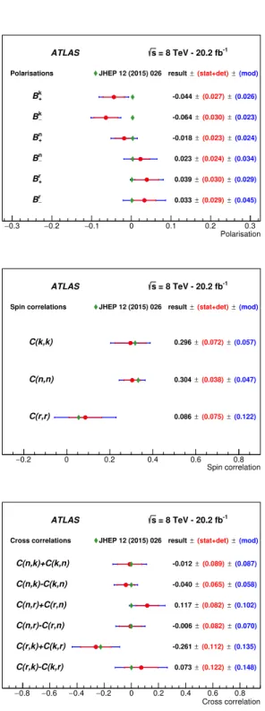
. Figure

5

shows the predictions at 8 TeV calculated in

ref. [

19

] and the unfolded result. None of the observables deviate significantly from the SM

predictions. The transverse correlation, C(n, n), differs from the case of no spin correlation

by 5.1 standard deviations. The correlations between the different polarisation and spin

correlations were evaluated and found to be small. The highest correlations are found to

be around 10% between the polarisation and spin correlation along the helicity axis and

the r-axis and between some cross correlations.

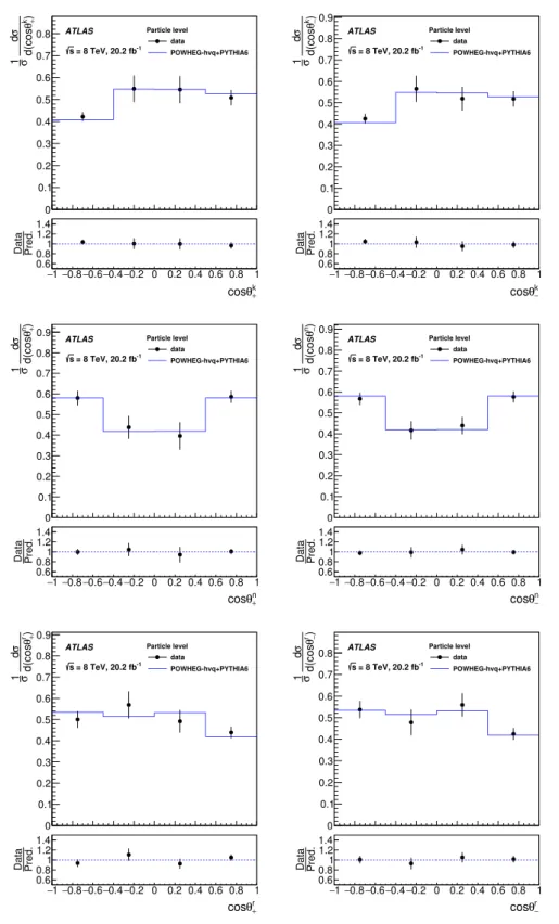
Figures

6

to

8

show the observable distributions corrected back to stable-particle level

and compared to the generated distribution created from Powheg-hvq +Pythia6. No

significant difference between the shapes of the observed and predicted distributions is

observed. The means of the distributions are compared between unfolded data and MC

predictions. They are presented in table

5

. In order to compare the size of the uncertainties

with the parton level measurement, the means of the polarisation observables are multiplied

by a factor of 3 and the correlations by a factor of −9 (section

3

). Overall the total

uncertainties for the measurements at parton and particle level are comparable. The mass

uncertainty is shown separately and not added to the total uncertainty, as explained in

section

6.3

. The dependence of the measured polarisations and spin correlations on the

MC top quark mass is presented in table

6

. The measurements presented in this paper are

compatible with other direct measurements in terms of central values and uncertainties for

the polarisations along the helicity and transverse axis as well as for the spin correlation

along the helicity axis (table

7

).

JHEP03(2017)113

Measurements Central Total Statistical Detector Modelling Others Mass

Full phase-space

B+k −0.044 ±0.038 ±0.018 ±0.001 ±0.026 ±0.007 ±0.027 B−k −0.064 ±0.040 ±0.020 ±0.001 ±0.023 ±0.014 ±0.027 B+n −0.018 ±0.034 ±0.020 ±0.001 ±0.024 ±0.005 -Bn − 0.023 ±0.042 ±0.020 ±0.001 ±0.034 ±0.005 -Br + 0.039 ±0.042 ±0.026 ±0.001 ±0.029 ±0.005 -B−r 0.033 ±0.054 ±0.023 ±0.002 ±0.045 ±0.006 ±0.016 C(k, k) 0.296 ±0.093 ±0.052 ±0.006 ±0.057 ±0.011 ±0.037 C(n, n) 0.304 ±0.060 ±0.028 ±0.001 ±0.047 ±0.001 ±0.010 C(r, r) 0.086 ±0.144 ±0.055 ±0.005 ±0.122 ±0.016 ±0.038 C(n, k) + C(k, n) −0.012 ±0.128 ±0.072 ±0.005 ±0.087 ±0.029 -C(n, k) − C(k, n) −0.040 ±0.087 ±0.053 ±0.004 ±0.058 ±0.003 -C(n, r) + C(r, n) 0.117 ±0.132 ±0.070 ±0.003 ±0.102 ±0.010 ±0.010 C(n, r) − C(r, n) −0.006 ±0.108 ±0.069 ±0.005 ±0.070 ±0.004 ±0.043 C(r, k) + C(k, r) −0.261 ±0.176 ±0.083 ±0.006 ±0.135 ±0.011 ±0.065 C(r, k) − C(k, r) 0.073 ±0.192 ±0.087 ±0.007 ±0.148 ±0.005 ±0.025

Fiducial phase-space

3hcos θk+i 0.125 ±0.044 ±0.018 ±0.007 ±0.025 ±0.020 ±0.027 3hcos θk−i 0.119 ±0.040 ±0.022 ±0.008 ±0.021 ±0.014 ±0.027 3hcos θn+i −0.025 ±0.042 ±0.024 ±0.001 ±0.027 ±0.005 -3hcos θn −i 0.023 ±0.046 ±0.024 ±0.001 ±0.036 ±0.006 -3hcos θr +i −0.104 ±0.045 ±0.027 ±0.008 ±0.030 ±0.006 -3hcos θr−i −0.110 ±0.060 ±0.024 ±0.008 ±0.050 ±0.010 ±0.015 -9hcos θk+cos θk−i 0.172 ±0.078 ±0.041 ±0.016 ±0.050 ±0.017 ±0.027 -9hcos θn+cos θn−i 0.427 ±0.079 ±0.034 ±0.011 ±0.065 ±0.004 ±0.027 -9hcos θr +cos θr−i 0.031 ±0.144 ±0.055 ±0.005 ±0.124 ±0.020 ±0.033 -9hcos θn

+cos θ−k + cos θk+cos θ−ni 0.024 ±0.132 ±0.078 ±0.004 ±0.085 ±0.025

--9hcos θn+cos θ−k − cos θk+cos θn−i −0.047 ±0.096 ±0.059 ±0.004 ±0.065 ±0.002

--9hcos θn+cos θ−r + cos θr+cos θn−i 0.113 ±0.143 ±0.076 ±0.005 ±0.108 ±0.023 ±0.015

-9hcos θn

+cos θ−r − cos θr+cos θn−i −0.030 ±0.118 ±0.076 ±0.005 ±0.077 ±0.007 ±0.052

-9hcos θr

+cos θ−k + cos θk+cos θr−i −0.187 ±0.151 ±0.069 ±0.023 ±0.122 ±0.006 ±0.039

-9hcos θr+cos θ k

−− cos θk+cos θ r

−i 0.047 ±0.128 ±0.070 ±0.003 ±0.082 ±0.010 ±0.023

Table 5. Results corrected to parton level in the full phase-space and to stable-particle level in the fiducial phase-space. The central value with the total uncertainty is shown as well as the contribution from the various systematic uncertainty categories. The uncertainty from the “Background” cate-gory is not shown because it is always smaller than 0.001. The total uncertainty corresponds to the sum in quadrature of the uncertainty obtained from the unfolding procedure with marginalisation (including the background and detector modelling), the signal modelling and the “Others” category. The numbers shown for the “Detector” category correspond to the sum in quadrature of the individ-ual estimates obtained as described in section6.3. The sum in quadrature of the values in the various columns thus does not necessarily match with the total uncertainty. The uncertainty related to the top quark mass is presented separately. It is shown as “-” when found to be compatible with zero.

JHEP03(2017)113

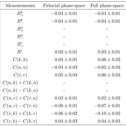
Measurements

Fiducial phase-space

Full phase-space

B

k +

−0.04 ± 0.01

−0.04 ± 0.01

B

₋k

−0.04 ± 0.01

−0.04 ± 0.01

B

₊n

-

-B

−n

-

-B

₊r

-

-B

−r

0.02 ± 0.01

0.03 ± 0.01

C(k, k)

0.04 ± 0.01

0.06 ± 0.02

C(n, n)

−0.04 ± 0.03

−0.02 ± 0.03

C(r, r)

0.05 ± 0.03

0.06 ± 0.03

C(n, k) + C(k, n)

-

-C(n, k) − C(k, n)

-

-C(n, r) + C(r, n)

0.02 ± 0.01

0.02 ± 0.02

C(n, r) − C(r, n)

−0.08 ± 0.01

−0.07 ± 0.01

C(r, k) + C(k, r)

−0.06 ± 0.02

−0.10 ± 0.02

C(r, k) − C(k, r)

0.04 ± 0.03

0.04 ± 0.03

Table 6. Dependence of polarisation and spin correlation measurements on the MC top quark mass. The slope, computed from the reference value of 172.5 GeV, is indicated for each measurement with its statistical uncertainty in units of GeV−1. Slopes which are compatible with zero within the uncertainty are indicated with “-”.

Experiment √s Method Bk+ Bk− C(k, k) Bn+ B−n

ATLAS 8 TeV Unfolding −0.044±0.038 −0.064±0.040 0.296±0.093 −0.018±0.034 0.023±0.042

CMS [16] 8 TeV Unfolding −0.022 ± 0.058 0.278 ± 0.084 -

-ATLAS [11] 7 TeV Template fit −0.035 ± 0.040 - -

-ATLAS [10] 7 TeV Template fit - - 0.23 ± 0.09 -

-ATLAS [12] 7 TeV Unfolding - - 0.315 ± 0.078 -

-D0 [17] 1.96 TeV Template fit −0.102 ± 0.061 - 0.040 ± 0.034

Table 7. Direct measurements of polarisations or spin correlations for different experiments and measurement techniques. If more than one measurement from an experiment is performed with the same technique, the measurement with the smallest total uncertainty is shown. If a measurement quotes polarisation values for a CP-conserving and a CP-violating production mechanism, the result for the CP-conserving case is shown in the table (P and C denote the parity and charge-conjugation transformations, respectively). The template fits for the polarisation observables usually use the information of both the top and antitop quark decay chains. In this case, only one polarisation value can be quoted as the result and is shown for both columns of polarisation along the same axis. The SM predictions of the polarisations at the Tevatron are slightly different [17, 72] due to the different dominant production mechanism, which is q ¯q annihilation. Dashes indicate no measurement for the corresponding analysis.

JHEP03(2017)113

Polarisation 0.3 − ₋0.2 ₋0.1 0 0.1 0.2 0.3 ATLAS k + B k − B n + B n − B r + B r − B

Polarisations JHEP 12 (2015) 026 result ±(stat+det)±(mod) (0.026) ± (0.027) ± -0.044 (0.023) ± (0.030) ± -0.064 (0.024) ± (0.023) ± -0.018 (0.034) ± (0.024) ± 0.023 (0.029) ± (0.030) ± 0.039 (0.045) ± (0.029) ± 0.033 -1 = 8 TeV - 20.2 fb s Spin correlation 0.2 − 0 0.2 0.4 0.6 0.8 ATLAS C(k,k) C(n,n) C(r,r)

Spin correlations JHEP 12 (2015) 026 result ±(stat+det)±(mod)

(0.057) ± (0.072) ± 0.296 (0.047) ± (0.038) ± 0.304 (0.122) ± (0.075) ± 0.086 -1 = 8 TeV - 20.2 fb s Cross correlation 0.8 − ₋0.6 ₋0.4 ₋0.2 0 0.2 0.4 0.6 0.8 ATLAS C(n,k)+C(k,n) C(n,k)-C(k,n) C(n,r)+C(r,n) C(n,r)-C(r,n) C(r,k)+C(k,r) C(r,k)-C(k,r)

Cross correlations JHEP 12 (2015) 026 result ±(stat+det)±(mod) (0.087) ± (0.089) ± -0.012 (0.058) ± (0.065) ± -0.040 (0.102) ± (0.082) ± 0.117 (0.070) ± (0.082) ± -0.006 (0.135) ± (0.112) ± -0.261 (0.148) ± (0.122) ± 0.073 -1 = 8 TeV - 20.2 fb s

Figure 5. Comparison of the measured polarisations and spin correlations (data points) with predictions from the SM (diamonds) for the parton-level measurement. Inner bars indicate uncer-tainties obtained from the marginalisation, outer bars indicate modelling systematics, summed in quadrature. The widths of the diamonds are chosen for illustrative purposes only.