Alfalfa reference crop evapotranspiration in Colorado and its use for irrigation scheduling

(1)

DISSERTATION

ALFALFA REFERENCE CROP EVAPOTRANSPIRATION IN COLORADO AND ITS USE FOR IRRIGATION SCHEDULING

Submitted by

Abdulkariem Mukhtar Aljrbi Department of Soil and Crop Sciences

In partial fulfillment of the requirements For the Degree of Doctor of Philosophy

Colorado State University Fort Collins, Colorado

Spring 2015

Doctoral Committee:

Advisor: Jessica G. Davis Co-Advisor: Allan A. Andales Yaling Qian

(2)

i

(3)

ii

ABSTRACT

ALFALFA REFERENCE CROP EVAPOTRANSPIRATION IN COLORADO AND ITS USE FOR IRRIGATION SCHEDULING

The goal of irrigation scheduling is efficient use of water such that water is applied to the field for optimal crop production. Previous studies have optimized irrigation scheduling using different models to manage sprinkler irrigation. This research evaluated approaches for obtaining alfalfa reference evapotranspiration (ETr) and its use in a new irrigation scheduling model for a furrow irrigation system. The objectives of this research were to: 1) Compare seasonal trends of daily ETr from the American Society of Civil Engineers Standardized Penman-Monteith (ASCE-SPM) equation and the Penman-Kimberly (PK) equation along a climatic gradient in Colorado, 2) Verify the agreement between calculated ETr from the ASCE-SPM equation and measured ETr from a lysimeter during the 2010 season for the Arkansas Valley of Colorado and correct the lysimeter ETr for alfalfa overgrowth, and 3) Test the ASCE-SPM ETr along with a locally adapted Kcr curve for corn in an irrigation scheduling spreadsheet tool for simulating the daily soil water deficit of furrow irrigated corn in northeast Colorado.

The two reference ET equations were compared using R2, Root-Mean-Square Error (RMSE), Relative Error (RE), and index of agreement (d). The R2 values ranged from 0.93 to 0.99; d ranged from 0.98 to 0.99, RMSE ranged from 0.29 to 0.75 mm/d, and RE ranged from -6.35 to 1.91 %. In a comparison of the ASCE-SPM and PK equations at the Fort Collins and

(4)

iii

Rogers Mesa sites in 2011, differences were observed between the energy balance and aerodynamic terms of each equation. The energy budget calculated by the ASCE-SPM was generally 28% lower than the energy budget calculated by the PK equation at both locations for 2011. On the other hand, the aerodynamic term calculated by the ASCE-SPM equation was from 27 – 28 % higher than the aerodynamic term calculated from PK during most of 2011 at both locations.

The second objective of this research compared alfalfa ET measured with a lysimeter in the center of a 4.06 ha furrow irrigated field at the Colorado State University Arkansas Valley Research Center in Rocky Ford, CO to the calculated values from the ASCE-SPM equation in periods of reference conditions in 2010. Four days were selected when alfalfa in the lysimeter was 50 – 55 cmtall, unstressed, completely covering the ground, but with its canopy extending beyond the outer walls of the lysimeter. On these dates, hourly lysimeter ETr was 0.08 to 0.11 mm/h higher than ASCE-SPM ETr. The theoretical surface area of the lysimeter was 9.181 m2, while the observed effective canopy area was up to 12.461 m2 due to overgrowth. Surface area corrections for the overgrowth increased the index of agreement (d) between hourly lysimeter ETr and ASCE-SPM ETr from the 0.96 – 0.98 range to the 0.99 – 1.0 range. These results showed that it is important to use the correct effective canopy area when computing ETr from a weighing lysimeter.

The CIS model for calculating water deficit under a furrow irrigation system with the addition of some data from field measurements such as soil moisture content, gross irrigation, climate data, and plant height and leaf area index generated good results. The water deficit under corn was simulated at the Limited Irrigation Research Farm (LIRF) located near Greeley,

(5)

iv

Colorado during the years 2010, 2011 and 2012. Daily corn crop ET (ETc) calculated from daily ASCE-SPM ETr and a locally-derived crop coefficient curve (Kcr) were used by the CIS for daily soil water deficit calculations via water balance. This data was used to test a furrow irrigation system via the CIS model and to simulate the field irrigation by predicting the time and the amount of water for the next irrigation. The results showed good agreement between calculated and measured deficits where index of agreement (d) ranged from 0.5 to 0.99 for most years of this study, specifically when measurements of soil water content (SWC) were inserted bi-weekly or monthly. The RMSE did not exceed 2.54 mm when using SWC once per season in 2011, while bi-weekly measurements recorded d to be 0.96 in 2010, 0.99 in 2011 and 0.70 in 2012. Also, the CIS showed that irrigation water usage could be reduced by 30 to 50% through use of CIS.

(6)

v

TABLE OF CONTENTS

ABSTRACT ... ii

TABLE OF CONTENTS ... iv

CHAPTER ONE: Introduction ... 1

References ... 6

CHAPTER TWO: Comparison of Reference Evapotranspiration Using the American Society of Civil Engineers (ASCE) Standardized Penman-Monteith and Penman-Kimberly Equations Across a Climatic Gradient in Colorado ... 10

Overview ... 10

Introduction... 11

Materials and Methods ... 13

Locations ... 13

Climatic data collection ... 13

ETr calculated by the American Society of Civil Engineers (ASCE) standardized Penman-Monteith Equation ... 14

ETr calculated by the Penman-Kimberly Equation ... 15

Terms of the ASCE-SPM and PK Equations... 16

Data processing ... 17

Evaluation and statistical analysis ... 17

Results and Discussion ... 19

Annual comparisons... 19

Daily differences by time of year ... 20

Differences in energy budget terms and aerodynamic terms ... 21

Effects of weather ... 22

Implications on crop coefficient curves ... 23

Conclusion ... 24

References ... 26

CHAPTER THREE: Effective Surface Area Corrections for Alfalfa Reference Evapotranspiration from a Weighing Lysimeter ... 46

(7)

vi

Location of lysimeter... 51

Lysimeter design ... 51

Measured evapotranspiration from lysimeter ... 52

The ASCE standardized reference equation ... 53

Lysimeter evapotranspiration corrections ... 54

Statistical analysis ... 55

Conclusion ... 60

References ... 61

CHAPTER FOUR: Evaluation of Colorado Irrigation Scheduler (CIS) for Furrow Irrigated Corn in Northeast Colorado ... 70

Overview ... 70

Field study ... 75

Soil water and crop measurement... 76

Evapotranspiration estimation... 77

Colorado Irrigation Scheduler (CIS) ... 81

CIS evaluation ... 83

Field water balance and corn growth ... 84

CIS evaluation ... 86

Conclusion ... 89

References ... 91

(8)

1 CHAPTER ONE: INTRODUCTION

The agriculture sector is the biggest water consumer in most countries that are interested in increasing agricultural production (Rosegrant et al., 2002). The competition for water resources from other sectors, such as municipal, has become one of the greatest challenges facing agricultural production (Rahaman and Varis, 2005). The rapid growth in population is accompanied by an increase in food demand and a reduction in the water quota for the agricultural sector (Bilsborrow, 1987). Under such conditions, it is important to use irrigation water more efficiently (Sinclair et al., 1984). Therefore, irrigation management increasingly relies on highly efficient tools to help reduce water use in agriculture (Cifre et al., 2005).

Evapotranspiration (ET) is the amount of water lost from plants and soils (Reynolds et al., 2004). The amount of water transpiration from plants into the atmosphere via stomata depends on water potential, humidity, availability of water in the soil, atmospheric moisture, and the temperature in the air and soil (Satoh et al., 2013). Plants use transpiration to cool plant cells (Han and Young, 2014). The climate plays an important role in controlling ET through factors such as solar radiation, temperature, wind, humidity and vapor pressure (Irmak et al., 2012). Water requirements depend on the evapotranspiration rate (Lopes and Bonaccurso, 2012). The quantity of water used for the synthesis of plant tissue is only 1% of the water absorbed, and the rest is lost by transpiration or water vapor which is not included in the processes of growth (Briggs and Smithson, 1986). The total amount of water which is needed by plants is very important in estimating the amount of irrigation water required in the different stages of plant life (Fereres and Soriano, 2007). The ET rate increases when soil water content is high because

(9)

2

more water is available to the plants (Van Donk et al., 2010). There is a direct correlation between evapotranspiration rate and soil water content, where higher ET rates are normally found after irrigation or precipitation due to availability of more water (Ferrante et al., 2014).

The ASCE standardized Penman-Monteith equation (ASCE-SPM) is one of many equations used to calculate evapotranspiration (Allen et al., 2005; Cobaner, 2011). Good results have been obtained from the ASCE-SPM equation during the reference stage when the plants are at standard height and without stress. The standardized reference ET can be calculated for (1) a short crop (similar to grass) or (2) a tall crop (similar to alfalfa) (Abtew and Melesse, 2013). ETos is the reference for short crops having a height of 12 cm, whereas ETrs is the reference for tall crops having a height of 50 cm. In addition, this equation can work in both hourly and daily time steps (Abtew and Melesse, 2013).

The best way to calculate crop ET from the field is with a lysimeter which provides precise crop ET measurements (López-Urrea et al., 2012). Precision weighing lysimeters are used to measure ET in the field using mass balance (Ding et al., 2010). Many studies have been conducted to compare measured ET using lysimeter data and calculated reference ET using 1982 Penman Kimberly (PK), FAO-56 Penman, and ASCE-SPM equations (Kumar et al., 2011). These studies concluded that all of those equations are sufficiently accurate to recommend their use for calculating reference evapotranspiration (Davidov and Moteva, 2010).

Increasing ET is a consequence of increasing water availability for consumption in the field (Chen et al., 2010). Irrigation management plays an important role in providing the

(10)

3

appropriate quantity of water to plants when needed (Hensley et al., 2011). Irrigation scheduling determines how much and when water is needed (Incrocci et al., 2014). Reducing water consumption in agriculture depends on irrigation management through irrigation scheduling (Knox et al., 2012). Irrigation scheduling focuses on when and how much water should be applied to the field before plants reach Management Allowed Depletion (MAD), and MAD is the amount of depletion of available water in the plant root zone (plant available water) that can be tolerated before applying water (Hillyer, 2011). Land should be irrigated so that soil water content is between field capacity and MAD and available to plants (Kumar et al., 2014).

Reference Evapotranspiration (Ref-ET) is a program

(http://www.kimberly.uidaho.edu/ref-et/) that can be used to calculate ETr, with inputs of

climatic data, and Colorado Agricultural Meteorological Network (CoAgMet) has been providing hourly and daily climate data since 1990 (Gleason, 2013). CoAgMet is also providing hourly and daily ET data using the ASCE-SPM and PK equations. Calculating accurate ET leads to obtaining good irrigation scheduling (Jayasinghe, 2013).

Accurate ETr leads to accurate crop ET (ETc) estimates, which are used in calculating the soil water balance for irrigation scheduling. ETc cannot be calculated without a crop coefficient (Kc). In Colorado the crop coefficients have been developed only for the PK equation (Gleason, 2013). The ETc equation follows

(11)

4

where ETc is crop evapotranspiration (mm/d); ETr is alfalfa reference evapotranspiration (mm/d) and Kcr is the alfalfa-based crop coefficient (Al Wahaibi, 2011). Gleason (2013) adapted a Kc curve for corn (Zea mays L.) for use with ASCE-SPM ETr under northeastern Colorado conditions.

Before using equation (1) for irrigation scheduling, one should test the accuracy of ETrs from the ASCE-SPM equation under field conditions because using untested ET could lead to inaccurate estimates of crop water requirement. The introduction of ETr from ASCE-SPM on the CoAgMet website has created a need to compare those values with the ETr from the PK equation under local Colorado climate conditions. Measured ETr from a lysimeter presents an actual ET from the field and can also be compared to ASCE-SPM ETr to verify their agreement.

The Colorado Irrigation Scheduler (CIS; Gleason, 2013) is a spreadsheet irrigation scheduling tool that uses the ASCE-SPM ETrs calculated by CoAgMet for estimating daily ETc. There is a need to test the CIS for furrow-irrigated fields in eastern Colorado. Furrow irrigation is a method of applying water at a specific rate of flow into shallow, evenly spaced channels (Burguete et al., 2014). Water is conveyed by these channels down the slope in the field, and plants can be planted either in the channels or on the beds between the channels depending on the agricultural practice in the region (Gonçalves et al., 2011). This method differs from flood irrigation in that only part of the ground surface is covered with water (Ebrahimian et al., 2013). The water moves through the soil both vertically and horizontally (Siyal et al. 2012). The furrow stream is applied until the desired application depth and lateral penetration are obtained (Ali, 2011). How long water must be applied in the furrows depends on the volume of water required

(12)

5

to fill the soil to the desired depth, the intake rate of the soil, and the spacing of the furrows and length of the field (Kelly et al., 2011). A uniform slope is preferred because this allows application of irrigation water with higher efficiency (Latif et al., 2013). Number of irrigation sets should be determined in the field, and the farm should be divided by set for irrigation. Also, time of application is the duration for which water is applied to the furrows in each set. The duration is the irrigation time period for each set to apply the required amount of water through each furrow at an acceptable irrigation efficiency (Reddy et al., 2013).

The objectives of this study were to:

1- Compare seasonal trends of daily ETr from the ASCE-SPM equation and the PK equation along a climatic gradient in Colorado.

2- Verify the agreement between calculated ETr from the ASCE-SPM equation and measured ETr from a lysimeter during the 2010 season for the Arkansas Valley of Colorado and correct the lysimeter ETr for alfalfa overgrowth.

3- Test the ASCE-SPM ETr along with a locally adapted Kcr curve for corn in an irrigation scheduling spreadsheet tool for simulating the daily soil water deficit of furrow irrigated corn in northeast Colorado.

(13)

6 References

Abtew, W., and A. Melesse. 2013. Reference and Crop Evapotranspiration. In Evaporation and Evapotranspiration. Springer, New York Volume 1 pp. 133-140.

http://link.springer.com/book/10.1007%2F978-94-007-4737-1

Al Wahaibi, H. S. 2011. Evaluating the ASCE Standardized Penman-Monteith Equation and Developing Crop Coefficients of Alfalfa Using a Weighing Lysimeter in Southeast Colorado Doctoral dissertation, Colorado State University, Fort Collins.

Ali, M. 2011. Irrigation System Designing. In Practices of Irrigation and On-farm Water

Management. Springer, New York. Volume 2 pp. 65-110.

http://link.springer.com/chapter/10.1007/978-1-4419-7637-6_3#page-1

Allen, R., Walter, I., Elliott, R., Howell, T., Itenfisu, D., Jensen, M., and Snyder, R. 2005. The ASCE standardized reference evapotranspiration equation, American Society of Civil Engineers. Environ. Water Resour. Inst., American Society of Civil Engineers, Reston, VA. Bilsborrow, R. E. 1987. Population pressures and agricultural development in developing

countries: A conceptual framework and recent evidence. World Development 15(2): 183-203.

Briggs, D. J., and P. Smithson. 1986. Fundamentals of Physical Geography. Rowman and Littlefield; London.

Burguete, J., Lacasta, A., and García-Navarro, P. 2014. SURCOS: A software tool to simulate irrigation and fertigation in isolated furrows and furrow networks. Computers and Electronics in Agriculture 103: 91-103.

Chen, L., Wang, J., Wei, W., Fu, B., and Wu, D. 2010. Effects of landscape restoration on soil water storage and water use in the Loess Plateau Region, China. Forest Ecology and Management 259(7): 1291-1298.

Cifre, J., Bota, J., Escalona, J. M., Medrano, H., and Flexas, J. 2005. Physiological tools for irrigation scheduling in grapevine (Vitis vinifera L.): An open gate to improve water-use efficiency? Agriculture, ecosystems and environment 106(2): 159-170.

Cobaner, M. 2011. Evapotranspiration estimation by two different neuro-fuzzy inference systems. Journal of Hydrology 398(3): 292-302.

Davidov, D., and M. Moteva. 2010. Comparison of crop evapotranspiration, calculated by FAO Penman-Monteith and by air temperature method. Agricultural Engineering 1: 102-106.

(14)

7

Ding, R., Kang, S., Li, F., Zhang, Y., Tong, L., and Sun, Q. 2010. Evaluating eddy covariance method by large-scale weighing lysimeter in a maize field of northwest China. Agricultural Water Management 98(1): 87-95.

Ebrahimian, H., Liaghat, A., Parsinejad, M., Playán, E., Abbasi, F., and Navabian, M. 2013. Simulation of 1D surface and 2D subsurface water flow and nitrate transport in alternate and conventional furrow fertigation. Irrigation Science 31(3): 301-316.

Fereres, E., and M. A. Soriano. 2007. Deficit irrigation for reducing agricultural water use. Journal of Experimental Botany 58(2): 147-159.

Ferrante, D., Oliva, G. E., and Fernández, R. J. 2014. Soil water dynamics, root systems, and plant responses in a semiarid grassland of Southern Patagonia. Journal of Arid Environments 104: 52-58.

Gleason, D.J. 2013. Evapotranspiration-based irrigation scheduling tools for use in eastern Colorado. M.S. Thesis, Colorado State University, Fort Collins.

Gonçalves, J. M., Muga, A. P., Horst, M. G., and Pereira, L. S. 2011. Furrow irrigation design with multicriteria analysis. Biosystems Engineering 109(4): 266-275.

Han, C., and S. L. Young. 2014. Drought and grazing disturbances and resistance to invasion by warm-and cool-season perennial grassland communities. Ecological Restoration 32(1): 28-36.

Hensley, M., Bennie, A. T. P., Van Rensburg, L. D., and Botha, J. J. 2011. Review of 'plant available water' aspects of water use efficiency under irrigated and dry land conditions. Water South Africa 37(5): 771-779.

Hillyer, C. C. 2011. Optimal Irrigation Management: A Framework, Model, and Application for Optimizing Irrigation when Supplies are Limited. Doctoral dissertation, Oregon State University, Corvallis.

Incrocci, L., Marzialetti, P., Incrocci, G., Di Vita, A., Balendonck, J., Bibbiani, C., and Pardossi, A. 2014. Substrate water status and evapotranspiration irrigation scheduling in heterogenous container nursery crops. Agricultural Water Management 131: 30-40.

Irmak, S., Kabenge, I., Skaggs, K. E., and Mutiibwa, D. 2012. Trend and magnitude of changes in climate variables and reference evapotranspiration over 116-yr period in the Platte River Basin, central Nebraska–USA. Journal of Hydrology 420: 228-244.

Jayasinghe, S. 2013. Evaluation of evapotranspiration methods to replace Penman-Monteith method in the absence of required climatic data in order to have a better irrigation scheduling. M.S. Thesis, University of Moratuwa, Sri Lanka.

(15)

8

Kelly, B. F. J., Acworth, R. I., and Greve, A. K. 2011. Better placement of soil moisture point measurements guided by 2D resistivity tomography for improved irrigation scheduling. Soil Research 49(6): 504-512.

Knox, J. W., Kay, M. G., and Weatherhead, E. K. 2012. Water regulation, crop production, and agricultural water management—Understanding farmer perspectives on irrigation efficiency. Agricultural Water Management 108: 3-8.

Kumar, B. A., Kanannavar, P., Balakrishnan, P., Pujari, B., and Hadimani, M. 2014. Laser guided land leveler for precision land development. Karnataka Journal of Agricultural Sciences 26(2):271-275.

Kumar, R., Shankar, V., and Kumar, M. 2011. Modelling of crop reference evapotranspiration: A review. Universal Journal of Environmental Research and Technology 1(3): 239-246. Latif, A., Shakir, A. S., and Rashid, M. U. 2013. Appraisal of economic impact of zero tillage,

laser land levelling and bed-furrow interventions in Punjab, Pakistan. Pak. J. Engineering and Applied Science 13: 65-81.

Lopes, M. C., and E. Bonaccurso. 2012. Evaporation control of sessile water drops by soft viscoelastic surfaces. Soft Matter 8(30): 7875-7881.

López-Urrea, R., Montoro, A., Mañas, F., López-Fuster, P., and Fereres, E. 2012. Evapotranspiration and crop coefficients from lysimeter measurements of mature ‘Tempranillo’wine grapes. Agricultural Water Management 112: 13-20.

Rahaman, M. M., and Varis, O. 2005. Integrated water resources management: evolution, prospects and future challenges. Sustainability: Science, Practice and Policy 1(1): 15-21. Reddy, J. M., Jumaboev, K., Matyakubov, B., and Eshmuratov, D. 2013. Evaluation of furrow

irrigation practices in Fergana Valley of Uzbekistan. Agricultural Water Management 117: 133-144.

Reynolds, J. F., Kemp, P. R., Ogle, K., and Fernández, R. J. 2004. Modifying the ‘pulse–reserve’ paradigm for deserts of North America: precipitation pulses, soil water, and plant responses. Oecologia 141(2): 194-210.

Rosegrant, M.W., X. Cai, and S.A. Cline. 2002. World water and food to 2025: dealing with scarcity. Joint publication of IFPRI, Washington DC, USA and International Water Management Institute (IWMI), Sri Lanka.

Satoh, T., Sugita, M., Yamanaka, T., Tsujimura, M., and Ishii, R. 2013. Water Dynamics within the Soil–Vegetation–Atmosphere System in a Steppe Region Covered by Shrubs and Herbaceous Plants. In: Yamamura, N., Fujita, N., Maekawa, A. (Eds.). The Mongolian

(16)

9

Network: Environmental Issues under Climate and Social Changes. Ecological Research Monographs. Springer, Tokyo. pp. 43–63. http://dx.doi.org/10.1007/978-4-431-54052-6_5

Sinclair, T. R., Tanner, C. B., and Bennett, J. M. 1984. Water-use efficiency in crop production. BioScience: PP. 36-40.

Siyal, A. A., Bristow, K. L., and Šimůnek, J. 2012. Minimizing nitrogen leaching from furrow irrigation through novel fertilizer placement and soil surface management strategies. Agricultural Water Management 115: 242-251.

Van Donk, S., Martin, D. L., Irmak, S., Melvin, S. R., Peterson, J., and Davison, D. 2010. Crop residue cover effects on evaporation, soil water content, and yield of deficit irrigated corn in West Central Nebraska.Transactions of the ASABE 53(6): 1787-1797.

(17)

10

CHAPTER TWO: COMPARISON OF REFERENCE EVAPOTRANSPIRATION USING THE AMERICAN SOCIETY OF CIVIL ENGINEERS (ASCE) STANDARDIZED PENMAN-MONTEITH AND PENMAN-KIMBERLY EQUATIONS ACROSS A CLIMATIC GRADIENT IN COLORADO

Overview

Reference evapotranspiration (ET) is used to represent atmospheric demand for water. The Colorado Agricultural Meteorological Network (CoAgMet) provides weather data used for calculating alfalfa reference crop ET (ETr) using the Penman Kimberly (PK) equation. Recently, CoAgMet has also started to provide alfalfa reference ET using the ASCE Standardized Penman-Monteith equation (ASCE-SPM). The objectives of this study were (1) to compare the alfalfa reference crop ET using the ACSE-SPM and the PK equations along a climatic gradient in Colorado and (2) to evaluate the effects of weather factors on the reference ET values from these two equations. Hourly weather data was collected and obtained from CoAgMet from seven weather stations located in Fort Collins, Greeley, Iliff, Fruita, Rogers Mesa, Rocky Ford, and Yellow Jacket during the years 2008 to 2011. This data was then used to calculate hourly reference ET using the two equations. The two reference ET equations were compared using R2, Root-Mean-Square Error (RMSE), Relative Error (RE), and index of agreement (d). The R2 values ranged from 0.93 to 0.99; d ranged from 0.98 to 0.99, RMSE ranged from 0.29 to 0.75 mm/d, and RE ranged from -6.35 to 1.91 %. The seasonal cumulative ETr calculated values using the PK equation were lower than the ASCE-SPM values on average. For 2011, the highest

(18)

11

mean value of relative humidity and lowest mean value of solar radiation were observed at the southernmost site (CSU Rogers Mesa) where the lowest mean ETr values were calculated among the seven sites. In a comparison of the ASCE-SPM and PK equations at the Fort Collins and Rogers Mesa sites in 2011, differences were observed between the energy balance and aerodynamic terms of each equation. The energy budget calculated by the ASCE-SPM was generally 28% lower than the energy budget calculated by the PK equation at both locations for 2011. On the other hand, the aerodynamic term calculated by the ASCE-SPM equation was from 27 – 28 % higher than the aerodynamic term calculated from PK during most of 2011 at both locations.

Introduction

Evapotranspiration can be determined directly using lysimeters or can be calculated using reference ET equations. The 1982 Penman-Kimberly (PK) and the American Society of Civil Engineers standardized Penman-Monteith (ASCE-SPM; ASCE-EWRI, 2005) equations for alfalfa (tall reference) are two of the most commonly utilized equations to calculate reference ET (Itenfisu et al., 2003). Crop evapotranspiration (ETc) can be determined by multiplying the reference ET by a crop coefficient. However, the relative performance of these two equations has not been widely tested in irrigated regions of Colorado.

Many studies have been conducted which compare the results between different reference ET equations, such as the 1982 Penman-Kimberly (PK) and ASCE-SPM approaches (Itenfisu et al., 2003). These studies have concluded that both of those equations are sufficiently accurate to recommend their use for calculation of reference ET. This study compares ETr values calculated

(19)

12

using the ASCE-SPM and PK equations under local weather conditions in Colorado because crop coefficient (Kc) values in CoAgMet were developed for use with PK ETr. The question is; are major adjustments to the Kc curves required for use with ASCE-SPM ETr? This can only be verified by comparing the ETr values from the ASCE-SPM and PK equations throughout the growing season.

The ASCE-SPM and the PK equations are used to calculate crop water requirements under local climate and soil conditions (Irmak et al., 2008). Using these equations with inaccurate or average data for weather, soil, and crop conditions will result in inaccurate ET calculations. This can lead to wrong estimates for crop water requirements (Yoder et al., 2005). However, using the standardized information on crop ET rates combined with knowledge of the local weather, soil, and crop conditions can help to determine more efficient irrigation amounts and scheduling (Amir and Martin, 2001). In Colorado, the Colorado Agriculture Meteorological Network (CoAgMet) (http://ccc.atmos.colostate.edu/~coagmet) provides local weather data (Gent and Schwartz, 2003). It provides hourly and daily climate data and calculated reference ET rates and uses both the PK and the ASCE SPM equations (Taghvaeian et al., 2012).

In 2010, Liu et al. (2010) published results from their comparison of the FAO PM and PK methods using climatic data from 1951 to 2007 in the Beijing area. Statistical analyses showed that the PK method had high correlation with the PM method and the lowest values of Root-Mean-Square Error (RMSE).

A study by the Agricultural and Food Engineering Department at the Indian Institute of Technology was done at the experimental farm, Kharagpur, India and found from comparisons

(20)

13

of the equations with lysimeter data that the Penman-Monteith equation (1965) gave the best result followed by 1982-PK, and the RMSE in all cases varied between 0.08 and 0.76 mm/d (Kashyap and Panda, 2001).

A comparison study can determine the impacts of using two different reference ET equations for estimating crop ET for the semi-arid conditions of Colorado. The objectives of this study were to:

1- Compare the seasonal behaviors of the ETr values from ACSE-SPM and PK equations across a climatic gradient in Colorado from 2008 to 2011.

2- Determine and evaluate the effects of climatic factors on ETr and explain the differences between ASCE-SPM and PK ETr values.

Materials and Methods

Locations

The weather stations from the Colorado Agriculture Meteorological Network (CoAgMet) used in the study includes seven field sites in Colorado (Table 2-1). The locations of these sites represent a climatic gradient from west to east of Colorado. The hourly data which was used to calculate the ASCE-SPM reference and the PK ET were provided by CoAgMet from 2008 to 2011 (http://ccc.atmos.colostate.edu/~coagmet/station_description.php).

Climatic data collection

Complete automatic weather stations present at the seven sites were used to obtain the factors needed in the ETr equations. Climatic data was recorded automatically every minute

(21)

14

using a data logger and then processed as hourly and daily output. The sensor used to measure rainfall was a TE525 tipping bucket rain-gauge located >1 m above the ground. A R.M. Young Wind Sentry (prop-anemometer) placed 2 m above the ground was used to measure wind speed and wind direction. A Vaisala HMP45C Probe placed 1.5 m above the ground was used to measure temperature and relative humidity. A Licor LI-200X Pyranometer placed ~2 m above the ground was used to measure solar radiation. CSI Model 107 Soil Temp Probe (thermistor) sensors were installed at 0.05 m and 0.15 m depths below the soil surface where two sensors were used; or at 0.1 m depth where only one sensor was used

(http://ccc.atmos.colostate.edu/~coagmet/station_description.php).

ETr calculated by the American Society of Civil Engineers (ASCE) standardized Penman-Monteith Equation

The standardized reference ET can be calculated for (1) a short crop (similar to grass) or (2) a tall crop (similar to alfalfa). ETos is the reference for a short crop that has a height of 12 cm whereas ETrs is the reference for a tall crop that has a height of 50 cm. In addition, this equation can work with both hourly and daily reference ET equations.

The ASCE-SPM equation for tall reference is given:

ET

rs

=

0.408 ∆ (Rn −G)+γ Cn

T+273 u2(es−ea)

∆+ γ(1+Cdu2)

Eq. (1)

where the units for the factor 0.408 coefficient is m2 mm/MJ. ETrs is the standardized reference crop ET for tall surfaces (mm/h); Δ is the slope of the saturation vapor pressure-temperature

(22)

15

curve (kPa/°C); Rn is the calculated net radiation at the crop surface (MJ/m2/h); G is the soil heat flux density at the soil surface (MJ/m2/h); γ is a psychrometric constant (kPa/°C); Cn is the numerator values that changes with reference type and calculation time step (K mm s3/Mg/h or K mm s3/Mg/d); T is the mean hourly air temperature in °C at 1.5 to 2.5-m height; u2 is the mean hourly wind speed at 2 m height (m/s); es is the saturation vapor pressure at 1.5 to 2.5 m height (kPa); ea is the mean actual vapor pressure at 1.5 to 2.5 m height (kPa); Cd is a denominator value that changes with reference type and calculation time step (s/m) (Allen et al., 2007). For this study, the ASCE-SPM was used to calculate hourly tall (alfalfa) reference ETrs. The standardized Cn and Cd values were Cn= 66 (K mm s3/Mg/h) at daytime and nighttime and Cd = 0.25 (s/m) at daytime and Cd = 1.7 (s/m) at nighttime.

ETr calculated by the Penman-Kimberly Equation

The following equation was used for hourly time steps:

λETr= _{∆+ γ} ∆ (Rn- G) +_{∆+ γ} γ 0.268(es − ea )Wf Eq. (2)

where ETr is the reference ET (mm h-1), λ is latent heat of vaporization (MJ kg-1) and Wf is the wind function. The wind function was calibrated for the Kimberly, Idaho locale, and the wind function coefficients vary with the time of year. Net radiation coefficients in the 1982 Penman-Kimberly also depend on the time of year. The Penman-Penman-Kimberly 1996 ETr values were calculated using the wind function (Wright et al., 2000).

The dimensionless wind function is calculated as follows:

(23)

16

where: aw and bw are empirical coefficients that lessen the effect of the wind function and they are calculated as follows with x representing the day number in the calendar year (Wright, 2000):

𝑎𝑤 = 0.4 + 1.4 ∗ 𝑒�−� 𝑥−173 58 � 2 � Eq. (4)

bw =0.007+0.004 ∗ 𝑒�−�𝑥−24380 � 2 � Eq. (5)

U2 is the wind speed at 2 m height in kilometers per day. Terms of the ASCE-SPM and PK equations

The Ref-ET program (Allen, 2000) is software used for calculating the reference ET rates from weather data and includes 15 methods, including the ASCE-SPM and the PK equations

(http://www.kimberly.uidaho.edu/ref-et/).

Ref-ET provides output of some terms of each equation that were used to calculate ETr. The aerodynamic term includes some weather data and canopy characteristics such as temperature, wind speed, vapor pressure, plant height, LAI, surface resistance and stomata resistance. The energy budget term includes net radiation and soil heat flux density at the soil surface (equations 1 and 2). Daily aerodynamic and energy budget terms were calculated separately from the ASCE-SPM and PK equations and then compared for the CSU ARDEC and Rogers Mesa Sites in 2011 to study the differences between the terms of both equations (ASCE-EWRI, 2005).

(24)

17 Data processing

The REF-ET computer program can calculate reference ET using 15 different equations, two of which are the ASCE-SPM and PK. This program was used to calculate reference ET for a tall crop (similar to alfalfa) that has a height of 50 cm. The calculations were based on the climate data that are available on CoAgMet. The hourly climatic data included Mean Temperature (oC), Vapor Pressure (kPa), Solar Radiation (MJ/m2), mean wind speed (m/s), and Mean of Relative Humidity (%). Four years of data (2008 - 2011) obtained from CoAgMet were transferred into Excel and then used by the Ref-ET program to calculate hourly reference evapotranspiration using ASCE-SPM and PK.

The comparisons between the two equations were made using the daily reference ET which was calculated in a 2 step process; hourly weather data were used to calculate hourly ETr, and then hourly ETr were summed for each 24-hour period to get daily ETr. This two-step process is deemed more accurate than using daily climate data in calculating the ETr directly (Allen, 2000).

Evaluation and statistical analysis

The calculated data were analyzed using Microsoft Office Excel. The regression lines of daily ETr calculated with the two equations were statistically analyzed for the seven locations and four years. The comparisons between the two equations were made using the daily readings to show the correlation and relationship between the ETr values.

(25)

18

Several statistics were used to compare the two ETr equations including Sum, Average, Minimum (Min), Maximum (Max), Standard Deviation (STDEV), and R2. In addition, Root-Mean-Square Error (RMSE) is a statistic used in environmental estimation models (Jacovides and Kontoyiannis, 1995; Wallach, 2006). Small RMSE values indicate good agreement. However, RMSE values are not a good indication of over or under estimation of a model (Jacovides and Kontoyiannis, 1995). Relative Error (RE) was used to present the percentage difference between ETr from the two equations (Willmott et al., 1985). The index of agreement (d) is another indicator used to measure performance of a model (Harmel and Smith, 2007). It has a domain between one and zero. A 1 value means an excellent agreement, while a 0 value means a poor agreement. Alternatively, R squared (R2) shows how well data points fit a line or curve. An R2 value of 1 means an excellent fitting line, while a 0 value means a poor fitting line (Cameron and Windmeijer, 1997).

Root-Mean-Square Error (RMSE) was calculated as follows:

RMSE = �1/N �(yi− xi)2 N 𝒾=1 � 1/2 Eq. (4)

where N is the total number of observations, yi is the calculated SPM ETr, and xi is the calculated PK ETr (Willmott et al., 1985).

Relative Error (RE) was calculated as follows:

RE = � yi− x_x i

(26)

19

where RE is relative error used to indicate the percentage difference. It can be positive or negative. Positive values mean the percentage of over-estimation, and negative values mean the percentage of under-estimation (Willmott et al., 1985). yi is mean ETr from PK equation and xi is mean ETr from ASCE-SPM equation.

Index of agreement (d) was calculated as follows:

d = 1 − �_{∑ (|y}∑ (yN𝒾=1 i− xi)2

i′| − |xi′|)2 N

𝒾=1 � Eq. (6)

where: d is between one and zero, y_i′= y_i − x� and x_i′= x_i − x� , yi and x� is the mean measured value (Willmott et al., 1985). yʹi is the ASCE-SPM values and xʹi is the PK values.

Results and Discussion

Annual comparisons

For each year, mean ETr values using the PK equation were always lower than the values obtained from the ASCE-SPM equation for all locations except the CSU Rogers Mesa site (Table 2-2). The values in the Index of Agreement were close to one (Table 2-2). The negative values for the Relative Error of Mean (%) indicate that the PK ETr is lower than the ASCE-SPM ETr on an annual basis. The R2 values (0.93 - 0.99) indicate that the ETr from the two equations were strongly correlated in each of the four years in all seven locations. The difference at CSU Expt Rocky Ford for 2011 was the highest compared to other years and other stations, where RE was at -6.4% and RMSE was at 0.72 mm/d (Table 2-2). The two equations have some differences in

(27)

20

the way the energy balance and aerodynamic terms are calculated, but the weather data used in both equations are the same, and they calculate daily ETr under similar conditions. The calculated ETr from the two equations showed that the PK equation generally resulted in lower annual or seasonal ETr values than the ASCE-SPM equation which illustrates an important difference between the equations. Based only on mean ETr values from ASCE-SPM equation and the most complete year of record (2011), the highest mean daily ETr was observed at Rocky Ford (5.26 mm/d) while the lowest was at Rogers Mesa (3.66 mm/d) (Table 2-3).

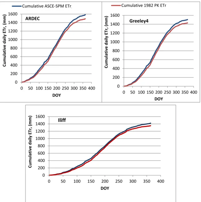
To show the cumulative differences throughout a season, daily cumulative plots are shown for all locations in 2011 (Figures 2-5 and 2-6). The cumulative daily ETr based on the ASCE-SPM and PK equations for 2011 in each of the seven locations was ideal in 2011 in terms of having a full weather data set. The cumulative reference ET data showed the correlation between the total readings of daily ETr based on the two equations for the years studied at the seven stations, but the cumulative reference ETr data from the two equations did not match during the year. The cumulative figures show that the PK values were generally lower than the ASCE-SPM. The CSU Rogers Mesa site showed the cumulative daily ETr based on the PK equation was very close to the cumulative daily ETr based on the ASCE-SPM equation.

Daily differences by time of year

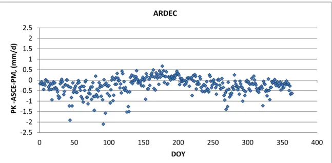
The differences between the calculated PK ET rates and the ASCE-SPM ET rates were least in the summer months (May - October) at the majority of the stations (Figures 2-7 to 2-13). The differences were greater in late winter and early spring months for all locations. Figures 2-7 to 2-13, for the years 2008, 2010, and 2011, show differences in the daily ETr values calculated

(28)

21

using the ASCE-SPM and PK equations for the seven locations. Note that the daily PK ETr was generally lower than the daily ASCE-SPM ETr during the spring, fall, and winter periods. The greatest differences were during spring months followed by the fall months at most locations. Figures 2-10 to 2-12 shows the largest differences in the daily ETr at the CSU Expt. Rocky station for winter 2011 while the lowest differences during this same period were at the CSU Rogers Mesa station. During the months May through October, the ETr for the two equations had a smaller difference than the months November through April (ASCE-EWRI, 2005).

Differences in energy budget terms and aerodynamic terms

Figure 2-14 shows a comparison of the daily energy budget terms (mm/d) as calculated by the ASCE-SPM and PK equations at CSU ARDEC Station and CSU Rogers Mesa station for 2011. At the ARDEC station the daily energy budget terms of the PK equation was higher than the daily energy budget terms of the ASCE-SPM equation during 2011. The ETr can be affected directly by net radiation and soil heat flux because they are the main factors in energy budget terms. Also, Figure 2-15 shows the difference between the aerodynamic part of calculating ETr from ASCE-SPM and PK equations. Aerodynamic term can be affected too by the weather and plant factors such as temperature, wind speed, humidity, vapor pressure, plant height, LAI, surfaces resistance of plant and stomata resistance. Therefore, at the CSU ARDEC Station and CSU Rogers Mesa station for 2011 show clear differences from calculating aerodynamic term by the two equations. The aerodynamic term calculated by the PK equation was generally lower than the aerodynamic term calculated by ASCE-SPM equation during the year. The differences in the energy budget term and aerodynamic term between the two equations explain why the

(29)

22

ASCE-SPM equation gave relatively higher ETr values than PK equation during the four years in most locations in Colorado.

Figure 2-16 shows greater variability in net radiation (Rn) differences between the two equations during winter, spring and fall periods; and the PK Rn values to be more consistently lower than ASCE-SPM Rn values from DOY 120 to 230 (mid-year). The differences between the PK and ASCE-SPM ETr appear to be correlated to the differences in net radiation when looking at these differences at the CSU ARDEC Station and CSU Rogers Mesa Station during 2011 (Figure 2-16; Figures 2-7 and 2-12). A small difference between net radiation as calculated by the two equations correlates to a small difference in ETr between the two equations. Likewise, a large difference between net radiation correlates to larger differences in ETr values from the two equations.

Effects of weather

The effects of weather parameters on ETr differences between the two equations are shown in Figures 2-17 to 2-20. There was no obvious trend in the differences versus Rn (Figure 2-17). However, the difference between PK and ASCE-SPM ETr became generally more negative when wind speeds were above 2 m/s (Figure 2-18).

The difference between PK and ASCE-SPM ETr was also affected by humidity (actual vapor pressure or relative humidity). The PK equation tended to give lower ETr values than the ASCE-SPM equation as vapor pressure or relative humidity decreased (Figures 2-19 and 2-20).

(30)

23

Differences in ETr were generally less than 0.5 mm/d when mean actual vapor pressure was higher than 1.5 kPa (Figure 2-19).

Implications on crop coefficient curves

Crop evapotranspiration (ETc) comprises most of the consumptive water use of plants. ETc can be calculated by multiplying ETr from ASCE-SPM equation or PK equation with a crop coefficient (Kc) that varies with growth stage. The Kc represents the characteristics of plants such as canopy cover, growth stage, leaf area index, and crop type that affect the amount of ETc. The length of each growth stage depends on the climate, latitude, elevation, planting date, and crop type, maturity group of different varieties or cultivars, and management practices.

Early in the growing season during the crop germination and establishment stage, most ETc occurs as evaporation from the soil surface. As the crop canopy develops and covers the soil surface, evaporation from the soil surface decreases and transpiration increases. Early in the season when the plant is small, the water use rate and Kc value also are small (Kc initial stage). As the plant develops, the crop ET rate increases. For agronomic plants, the crop ET rate is at the maximum level when the plant is fully developed (Kc mid-season). The ET rate decreases again toward the end of the season when the plant reaches physiological maturity (Kc end season).

Mean Kc values can be calculated by taking the ratio of measured ETc and calculated ETr from a reference ET equation, such as the PK or ASCE-SPM equation. In most locations in this study, the comparison between ETr values from the ASCE-SPM and PK equations showed generally lower ETr values from the PK equation. Thus, the lower ETr values from the PK

(31)

24

equation would result in higher calculated Kc values compared to using the ASCE-SPM equation. Given that the Kc values currently used in CoAgMet were developed for use with PK ETr values, those Kc values would generally have to be decreased in the spring and fall periods and increased during summer, before they can be used with the ASCE-SPM ETr values. Therefore, the development of new seasonal Kc curves for use with the ASCE-SPM ETr values is recommended for Colorado conditions.

Conclusion

The current analysis is a comprehensive comparison of the daily ETr values from the ASCE-SPM and PK equations. This analysis used hourly weather data gathered from seven different locations in Colorado. In general, the PK equation tended to give lower ETr values during spring and fall periods, and slightly higher values during summer months compared to the ASCE-SPM equation. Comparisons of the seasonal cumulative ETr showed that the PK equation values were consistently lower than the ASCE-SPM equation. The aerodynamic term calculated by the ASCE-SPM equation was generally higher than the aerodynamic term calculated by the PK equation, and the energy budget term calculated by the PK was generally higher than the energy budget term calculated by the ASCE-SPM equation. The behaviors of the daily energy budget and aerodynamic terms explain the reason why the ASCE-SPM ETr is relatively higher than PK ETr.

The difference between PK and ASCE-SPM ETr became generally more negative when wind speeds were above 2 m/s. The difference between PK and ASCE-SPM ETr was also affected by humidity (actual vapor pressure or relative humidity). The PK equation tended to give lower ETr values than the ASCE-SPM equation as vapor pressure or relative humidity

(32)

25

decreased. Differences in ETr were generally less than 0.5 mm/d when mean actual vapor pressure was higher than 1.5 kPa.

Given the differences in ETr values from the PK and the ASCE-SPM equations and the move towards adopting the ASCE-SPM equation in Colorado, it is recommended that new Kc curves for calculating ETc be developed for use with ASCE-SPM ETr values.

(33)

26 References

Allen, R.G. 2000. Ref-Et: Reference evapotranspiration calculation software for FAO and ASCE standardized equations, University of Idaho. Available online at:

www.kimberly.uidaho.edu/ref-et/ (accessed 7 March 2012).

Amir, K., And Martin, S. 2001. FAO Methodologies on Crop Water Use and Crop Water Productivity. Expert Meeting on Crop Water Productivity, Rome, Italy, 3–5 December 2001.

ASCE-EWRI. 2005. The ASCE standardized reference evapotranspiration equation. In: Allen RG, Walter IA, Elliot RL, et al. (eds.) Environmental and Water Resources Institute (EWRI) of the American Society of Civil. Engineers, ASCE, Standardization of Reference Evapotranspiration Task Committee Final Report, 213pp. Reston, VA: American Society of Civil Engineers (ASCE).

Cameron, A. C., and Windmeijer, F. A. 1997. An R-squared measure of goodness of fit for some common nonlinear regression models. Journal of Econometrics 77(2): 329-342.

Gent, D. H., and H. F. Schwartz. 2003. Validation of potato early blight disease forecast models for Colorado using various sources of meteorological data. Plant Disease 87(1): 78-84. Harmel, R.D., and Smith, P.K. 2007. Consideration of measurement uncertainty in the evaluation

of goodness-of-fit in hydrologic and water quality modeling. Journal of Hydrology 337: 326–336.

Irmak, A., Irmak, S., and Martin, D. L. 2008. Reference and crop evapotranspiration in south central Nebraska. I: Comparison and analysis of grass and alfalfa-reference evapotranspiration. Journal of Irrigation and Drainage Engineering 134(6): 690-699.

Itenfisu, D., Elliott, R. L., Allen, R. G., and Walter, I. A. 2003. Comparison of reference evapotranspiration calculations as part of the ASCE standardization effort. Journal of Irrigation and Drainage Engineering 129(6): 440-448.

Jacovides, C.P., and Kontoyiannis, H. 1995. Statistical procedures for the evaluation of evapotranspiration computing models. Agricultural Water Management 27: 365-371.

Kashyap, P. S., and R. K. Panda. 2001. Evaluation of evapotranspiration estimation methods and development of crop-coefficients for potato crop in a sub-humid region. Agricultural Water Management 50(1): 9-25.

Liu, Y., Liu, H. J., and Luo, Y. 2010. Comparison of potential evapotranspiration methods in Beijing area of China. Journal of Irrigation and Drainage 29(5): 27-32.

(34)

27

Taghvaeian, S., Chávez, J. L., and Hansen, N. C. 2012. Infrared thermometry to estimate crop water stress index and water use of irrigated maize in Northeastern Colorado. Remote Sensing 4(11): 3619-3637.

Wallach, D. 2006. Evaluation of crop models. In: D. Wallach, D. Makowski and J.W. Jones. Working with Dynamic Crop Models: Evaluation, Analysis, Parameterization and Applications, Elsevier, Amsterdam. pp. 11–53.

Willmott, C. J., Ackleson, S. G., Davis, R. E., Feddema, J. J., Klink, K. M., Legates, D. R., and Rowe, C. M. 1985. Statistics for the evaluation and comparison of models. Journal of Geophysical Research: Oceans (1978–2012) 90(C5): 8995-9005.

Wright, J.L., Allen, R.G., and Howell, T.A. 2000. Conversion between evapotranspiration references and methods. In: Proceedings of Fourth Decennial National Irrigation Symposium, Phoenix, AZ, ASAE, St. Joseph, MI, pp. 251–259.

Yoder, R. E., Odhiambo, L. O., and Wright, W. C. 2005. Evaluation of methods for estimating daily reference crop evapotranspiration at a site in the humid southeast United States. Applied Engineering in Agriculture 21(2): 197-202.

(35)

28

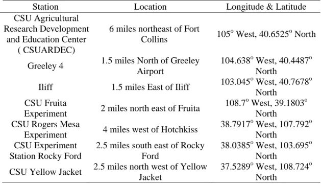
Table 2-1: The locations of the weather stations in Colorado which were used for comparison of ETr calculated by the ASCE-SPM and PK equations.

Station Location Longitude & Latitude

CSU Agricultural Research Development

and Education Center ( CSUARDEC)

6 miles northeast of Fort

Collins 105

o

West, 40.6525o North

Greeley 4 1.5 miles North of Greeley _Airport 104.638 o

Iliff 1.5 miles East of Iliff 103.045 o

CSU Fruita

Experiment 2 miles north east of Fruita

108.7o West, 39.1803o North

CSU Rogers Mesa

Experiment 4 miles west of Hotchkiss

38.7917o West, 107.792o North

CSU Experiment Station Rocky Ford

2.5 miles south east of Rocky Ford

38.0385o West, 103.695o North

CSU Yellow Jacket 2.5 miles north west of Yellow Jacket

37.5289o West, 108.724o North

(36)

29

Table 2-2: Statistical evaluation of the agreement of the two ETr calculations using the ASCE-SPM and PK equations at seven Colorado weather stations over four years. RE is Relative Error (%),RMSE is Root-Mean-Square Error (mm/d), d is Index of Agreement and R2 is R squared.

Year RE (yi =PK and xi =ASCE-SPM) (%) RMSE (mm/d) Index of Agreement (d) R 2 ARDEC 2008 -4.96 0.75 0.98 0.93 2009 -5.92 0.49 0.99 0.97 2010 -8.12 0.43 0.99 0.98 2011 -5.99 0.47 0.99 0.98 Greeley 2008 -0.76 0.34 0.99 0.99 2009 -1.03 0.33 0.99 0.98 2010 -3.27 0.36 0.99 0.99 2011 -4.94 0.44 0.99 0.98 Iliff 2008 -3.58 0.52 0.99 0.97 2009 -0.59 0.29 0.99 0.99 2010 -3.93 0.38 0.99 0.98 2011 -4.93 0.43 0.99 0.98

(37)

30

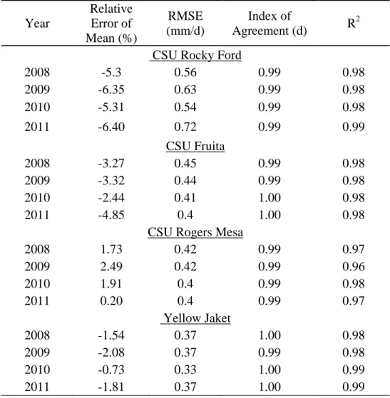
Table 2-2: Statistical evaluation of the agreement of the two ETr calculations using the standardized ASCE- PM ET and the PK at seven Colorado weather stations over four years. RE is Relative Error (%),RMSE is Root-Mean-Square Error (mm/d), d is Index of Agreement and R2 is R squared. (Continued) Year Relative Error of Mean (%) RMSE (mm/d) Index of Agreement (d) R 2

CSU Rocky Ford

2008 -5.3 0.56 0.99 0.98 2009 -6.35 0.63 0.99 0.98 2010 -5.31 0.54 0.99 0.98 2011 -6.40 0.72 0.99 0.99 CSU Fruita 2008 -3.27 0.45 0.99 0.98 2009 -3.32 0.44 0.99 0.98 2010 -2.44 0.41 1.00 0.98 2011 -4.85 0.4 1.00 0.98

CSU Rogers Mesa

2008 1.73 0.42 0.99 0.97 2009 2.49 0.42 0.99 0.96 2010 1.91 0.4 0.99 0.98 2011 0.20 0.4 0.99 0.97 Yellow Jaket 2008 -1.54 0.37 1.00 0.98 2009 -2.08 0.37 0.99 0.98 2010 -0.73 0.33 1.00 0.99 2011 -1.81 0.37 1.00 0.99

(38)

31

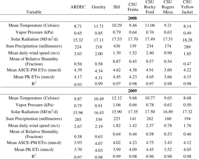
Table 2-3: Statistical summary of the climate input data and the daily ETr for the seven locations 2008 – 2011.The correlation (R2) indicates the strength of relationship between the daily ET values calculated by the standardized ASCE Penman Monteith and the Penman Kimberly equations. CSU is Colorado State University, and ARDEC is Agricultural Research Development and Education Center.

Variable

ARDEC Greeley Illif CSU Fruita CSU Rocky Ford CSU Rogers Mesa CSU Yellow Jacket 2008

Mean Temperature (Celsius) _8.71 _11.71 10.29 9.46 11.06 9.21 _8.14 Vapor Pressure (kPa) _0.65 _0.85 0.79 0.64 0.76 0.63 _0.49 Solar Radiation (MJ/m2/d) _15.32 _17.11 17.53 17.70 17.49 17.51 _18.28 Sum Precipitation (millimeters) ₂₂₄ ₂₁₈ 436 139 234 174 ₂₈₉

Mean daily wind speed (m/s) _3.03 _2.00 1.39 1.52 2.40 0.90 _1.85 Mean of Relative Humidity

(Fraction) 0.56 0.58 0.87 0.45 0.57 0.54 0.47 Mean ASCE-PM ETrs (mm/d) 4.39 _4.34 4.62 4.38 4.91 3.60 4.22 Mean PK ETrs (mm/d) 4.17 _4.31 4.45 4.23 4.65 3.66 4.15

R2 _0.93 0.99 0.97 0.98 0.97 0.98 0.98

2009

Mean Temperature (Celsius) _9.87 _10.49 12.12 9.68 10.77 9.63 8.68 Vapor Pressure (kPa) _0.75 _0.91 1.06 0.66 0.78 0.63 0.50 Solar Radiation (MJ/m2/d) _15.96 _16.43 15.90 17.35 17.50 16.89 17.32 Sum Precipitation (millimeters) ₂₈₅ ₃₃₉ 223 141 262 160 194

Mean daily wind speed (m/s) _2.67 _2.19 1.82 1.42 2.37 0.78 1.76 Mean of Relative Humidity

(Fraction) 0.58 0.63 0.64 0.46 0.58 0.53 0.46 Mean ASCE-PM ETrs (mm/d) 3.93 _4.07 4.02 4.23 4.75 3.43 4.12 Mean PK ETr (mm/d) 3.70 _4.03 3.99 4.09 4.45 3.52 4.03

(39)

32

Table 2-3: Statistical summary of the climate input data and the daily ETr for the seven locations 2008 – 2011.The correlation (R2) indicates the strength of relationship between the daily ET values calculated by the standardized ASCE Penman Monteith and the Penman Kimberly equations. CSU is Colorado State University, and ARDEC is Agricultural Research Development and Education Center. (Continued)

Variable

ARDEC Greeley Illif CSU Fruita CSU Rocky Ford CSU Rogers Mesa CSU Yellow Jacket 2010

Mean Temperature (Celsius) _13.20 _9.20 9.79 10.03 11.61 9.95 8.24 Vapor Pressure (kPa) _0.71 _0.75 0.84 0.72 0.80 0.64 0.58 Solar Radiation (MJ/m2/d) _16.03 _16.49 15.49 17.53 18.17 17.07 17.80 Sum Precipitation (millimeters) ₃₁₆ ₂₃₅ 379 206 346 309 293

R2 _0.98 _0.99 0.98 0.98 0.98 0.98 0.99

2011

Mean Temperature (Celsius) _8.86 _8.77 8.89 9.71 9.55 9.31 8.40 Vapor Pressure (kPa) _0.69 _0.73 0.82 0.71 0.68 0.61 0.54 Solar Radiation (MJ/m2/d) _16.01 _16.32 15.20 17.40 18.41 17.08 18.74 Sum Precipitation (millimeters) ₃₁₂ ₂₈₀ 492 214 153 267 312

(40)

33

Figure 2-1: Daily reference ET (mm/d) as calculated by the American Society of Civil Engineers Standardized Penman-Monteith (ASCE-SPM) and Penman-Kimberly (PK) equations at Agricultural Research Development and Education Center (ARDEC) and Iliff locations for 2008. DOY is day of year.

Figure 2-2: A comparison of the daily reference evapotranspiration (ETr, mm/d) as calculated by the American Society of Civil Engineers Standardized Penman-Monteith (ASCE-SPM) and Penman-Kimberly (PK) equations at the Greeley4 and Iliff locations for 2010. DOY is day of year. 0 2 4 6 8 10 12 0 50 100 150 200 250 300 350 400 (ET r , mm/d ) DOY Greeley 4 1982 PK ETr, (mm/d) ASCE-SPM ETr, (mm/d) 0 2 4 6 8 10 12 0 50 100 150 200 250 300 350 400 (ET r , mm/d ) DOY ASCE-SPM ETr, (mm/d) 1982 PK ETr, (mm/d) Ilif 0 2 4 6 8 10 12 0 50 100 150 200 250 300 350 (ET r , mm/d ) DOY ASCE-SPM ETr, (mm/d) 1982 PK ETr, (mm/d) Ilif 0 2 4 6 8 10 12 0 50 100 150 200 250 300 350 (ET r , mm/d ) DOY ASCE-SPM ETr, (mm/d) 1982 PK ETr, (mm/d) ARDEC

(41)

34

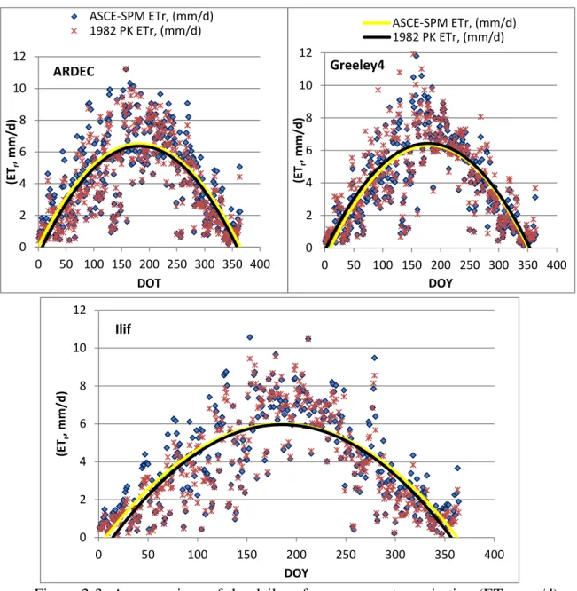
Figure 2-3: A comparison of the daily reference evapotranspiration (ETr, mm/d) as calculated by the American Society of Civil Engineers Standardized Penman-Monteith (ASCE-SPM) and Penman-Kimberly (PK) equations at Agricultural Research Development and Education Center (ARDEC), Greeley, and Iliff locations for 2011. DOY is day of year.

0 2 4 6 8 10 12 0 50 100 150 200 250 300 350 400 (ET r , mm/d ) DOY ASCE-SPM ETr, (mm/d) 1982 PK ETr, (mm/d) Greeley4 0 2 4 6 8 10 12 0 50 100 150 200 250 300 350 400 (ET r , mm/d ) DOY Ilif 0 2 4 6 8 10 12 0 50 100 150 200 250 300 350 400 (ET r , mm/d ) DOT ASCE-SPM ETr, (mm/d) 1982 PK ETr, (mm/d) ARDEC

(42)

35

Figure 2-4: A comparison of the daily reference evapotranspiration (ETr, mm/d) as calculated by the American Society of Civil Engineers Standardized Penman-Monteith (ASCE-SPM) and Penman-Kimberly (PK) equations at Colorado State University Fruita 02, at Colorado State University Rogers Mesa for 2011. DOY is day of year.

0 2 4 6 8 10 12 0 50 100 150 200 250 300 350 400 (ET r , mm/d ) DOY ASCE-SPM ETr, (mm/d) 1982 PK ETr, (mm/d) Yellow Jaket 0 2 4 6 8 10 12 0 50 100 150 200 250 300 350 400 (ET r , mm/d ) DOY Rogers mesa 0 2 4 6 8 10 12 0 50 100 150 200 250 300 350 400 (ET r , mm/d ) DOY Fruita 02 0 2 4 6 8 10 12 0 50 100 150 200 250 300 (ET r , mm/d ) DOY ASCE-SPM ETr, (mm/d) 1982 PK ETr, (mm/d) Roky Ford

(43)

36

Figure 2-5: Cumulative daily reference evapotranspiration (ETr, mm) calculated based on the American Society of Civil Engineers Standardized Penman-Monteith (ASCE-SPM) and Penman-Kimberly (PK) equations for 2011 from the Agricultural Research Development and Education Center (ARDEC), Greeley4, and Iliff stations. DOY is day of year.

0 200 400 600 800 1000 1200 1400 1600 0 50 100 150 200 250 300 350 400 Cu m ul ati ve da ily E Tr , ( m m ) DOY Iliff 0 200 400 600 800 1000 1200 1400 1600 0 50 100 150 200 250 300 350 400 Cu m ul ati ve da ily E Tr , ( m m ) DOY Cumulative 1982 PK ETr, (mm/d) Greeley4 0 200 400 600 800 1000 1200 1400 1600 0 50 100 150 200 250 300 350 400 Cu m ul ati ve da ily E Tr , ( m m ) DOY

Cumulative ASCE-SPM ETr, (mm/d) ARDEC

(44)

37 ‘

Figure 2-6: Cumulative daily reference evapotranspiration (ETr, mm) calculated based on the American Society of Civil Engineers Standardized Penman-Monteith (ASCE-SPM) and Penman-Kimberly (PK) equations for 2011 from the Colorado State University (CSU) Experiment Rocky Ford, CSU Fruita 02 Experiment station, CSU Rogers Mesa and Yellow Jacket stations. DOY is day of year.

0 200 400 600 800 1000 1200 1400 1600 0 50 100 150 200 250 300 350 400 Cu m ul ati ve da ily E Tr , ( m m ) DOY Yellow Jacket Cumulative 1982 PK ETr, (mm/d) 0 200 400 600 800 1000 1200 1400 1600 0 50 100 150 200 250 300 350 400 Cu m ul ati ve da ily E Tr , ( m m ) DOY

Cumulative ASCE-SPM ETr, (mm/d) Roky Ford 0 200 400 600 800 1000 1200 1400 1600 0 50 100 150 200 250 300 350 400 Cu m ul ati ve da ily E Tr , ( m m ) DOY Fruita 02 0 200 400 600 800 1000 1200 1400 1600 0 50 100 150 200 250 300 350 400 Cu m ul ati ve da ily E Tr , ( m m ) DOY Rogers Mesa

(45)

38

Figure 2-7: The difference in daily reference evapotranspiration (ETr, mm/d) between the Kimberly (PK) and the American Society of Civil Engineers Standardized Penman-Monteith (ASCE-SPM) equations from the Agricultural Research Development and Education Center (ARDEC) for 2011. DOY is day of year.

Figure 2-8: The difference in daily reference evapotranspiration (ETr, mm/d) between the Kimberly (PK) and the American Society of Civil Engineers Standardized Penman-Monteith (ASCE-SPM) equations from the Greeley4 station for 2011. DOY is day of year.

-2.5 -2 -1.5 -1 -0.5 0 0.5 1 1.5 2 2.5 0 50 100 150 200 250 300 350 400 P K -A SCE -P M, (m m /d ) DOY Greeley -2.5 -2 -1.5 -1 -0.5 0 0.5 1 1.5 2 2.5 0 50 100 150 200 250 300 350 400 P K -A SCE -PM , ( mm/d ) DOY ARDEC

(46)

39

Figure 2-9: The difference in reference evapotranspiration (ETr, mm/d) between the Penman-Kimberly (PK) and the American Society of Civil Engineers Standardized Penman-Monteith (ASCE-SPM) equations from the Iliff station for 2011. DOY is day of year.

Figure 2-10: The difference in daily reference evapotranspiration (ETr, mm/d) between the Penman-Kimberly (PK) and the American Society of Civil Engineers Standardized Penman-Monteith (ASCE-SPM) equations from the CSU Experiment Rocky station for 2011. DOY is day of year.

-2.5 -2 -1.5 -1 -0.5 0 0.5 1 1.5 2 2.5 0 50 100 150 200 250 300 350 400 P K -A SCE -P M, (m m /d ) DOY

CSU Expt. Rocky Ford -2.5 -2 -1.5 -1 -0.5 0 0.5 1 1.5 2 2.5 0 50 100 150 200 250 300 350 400 P K -A SCE -PM , ( mm/d ) DOY Ilif

(47)

40

Figure 2-11: The difference in daily reference evapotranspiration (ETr, mm/d) between the Kimberly (PK) and the American Society of Civil Engineers Standardized Penman-Monteith (ASCE-SPM) equations from the CSU Fruita Experiment station for 2011. DOY is day of year.

Figure 2-12: The difference in daily reference evapotranspiration (ETr, mm/d) between the Kimberly (PK) and the American Society of Civil Engineers Standardized Penman-Monteith (ASCE-SPM) equations from the Colorado State University Rogers Mesa station for 2011. DOY is day of year.

-2.5 -2 -1.5 -1 -0.5 0 0.5 1 1.5 2 2.5 0 50 100 150 200 250 300 350 400 P K -A SCE -P M, (m m /d ) DOY

CSU Rogers Mesa -2.5 -2 -1.5 -1 -0.5 0 0.5 1 1.5 2 2.5 0 50 100 150 200 250 300 350 400 P K -A SCE -PM , ( mm/d ) DOY CSU Fruita

(48)

41

Figure 2-13: The difference in daily reference evapotranspiration (ETr, mm/d) between the Kimberly (PK) and the American Society of Civil Engineers Standardized Penman-Monteith (ASCE-SPM) equations from the Yellow Jacket station for 2011. DOY is day of year.

-2.5 -2 -1.5 -1 -0.5 0 0.5 1 1.5 2 2.5 0 50 100 150 200 250 300 350 400 P K -A SCE -PM , ( mm/d ) DOY Yellow Jacket

(49)

42

Figure 2-14: A comparison of the daily energy budget term (mm/d) as calculated by the Penman-Kimberly (PK) and the American Society of Civil Engineers Standardized Penman-Monteith (ASCE-SPM) equations at the Agricultural Research Development and Education Center (ARDEC) and Colorado State University Rogers mesa stations for 2011. DOY is day of year.

Figure 2-15: A comparison of the daily aerodynamic term (mm/d) as calculated by the Penman-Kimberly (PK) and the American Society of Civil Engineers Standardized Penman-Monteith (ASCE-SPM) equations at the Agricultural Research Development and Education Center (ARDEC) and Colorado State University Rogers mesa stations for 2011. DOY is day of year.

0 1 2 3 4 5 6 7 8 9 10 0 50 100 150 200 250 300 350 400 Ae rod yn ami c T er m, (mm/d ) DOY Aerodynamic TermPM Aerodynamic TermPK Rogers 0 1 2 3 4 5 6 7 8 9 10 0 50 100 150 200 250 300 350 400 Ae rod yn ami c T er m, (mm/d ) DOY Aerodynamic TermPM Aerodynamic TermPK ARDEC 0 1 2 3 4 5 6 0 50 100 150 200 250 300 350 400 En er gy T er m , ( m m /d ) DOY Energy TermPK Energy TermPM Rogers 0 1 2 3 4 5 6 0 50 100 150 200 250 300 350 400 En er gy T er m , ( m m /d ) DOY Energy TermPK Energy TermPM ARDEC

(50)

43

Figure 2-16: The difference in daily net radiation (Rn, MJ/m2/d) as calculated by the Penman-Kimberly (PK) and the American Society of Civil Engineers Standardized Penman-Monteith (ASCE-SPM) equations at the Agricultural Research Development and Education Center (ARDEC) and Colorado State University Rogers mesa stations for 2011. DOY is day of year.

Figure 2-17: A comparison of the difference between daily reference evapotranspiration (ETr, mm/d) between the Penman-Kimberly (PK) and the American Society of Civil Engineers Standardized Penman-Monteith (ASCE-SPM) equations as affected by net radiation (Rn, Mj/m2/d) at CSU ARDEC and CSU Rogers mesa Stations for 2011.

-2 -1.5 -1 -0.5 0 0.5 1 1.5 0 50 100 150 200 250 300 350 400 Rn (P K-AS CE -SP M DOY Rn, (MJ/m^2/d) Rogers Rn, (MJ/m^2/d)ARDEC -3.5 -2.5 -1.5 -0.5 0.5 1.5 2.5 3.5 0 5 10 15 20 PK -A SCE -SP M, (m m /d ) Rn, (MJ/m2_/d) Rn, (MJ/m^2/d) Rogers -3.5 -2.5 -1.5 -0.5 0.5 1.5 2.5 3.5 0 5 10 15 20 PK -A SCE -SP M, (m m /d ) Rn, (MJ/m2_/d) Rn, (MJ/m^2/d) ARDEC