Measurement of hadronic event shapes in high-p(T) multijet final states at √s=13 TeV with the ATLAS detector

JHEP01(2021)188

Published for SISSA by Springer

Received: July 27, 2020 Revised: December 2, 2020 Accepted: December 14, 2020 Published: January 28, 2021

Measurement of hadronic event shapes in high-p

_T

multijet final states at

√

s = 13 TeV with the ATLAS

detector

The ATLAS collaboration

E-mail:

atlas.publications@cern.ch

Abstract: A measurement of event-shape variables in proton-proton collisions at large

momentum transfer is presented using data collected at

√

s = 13 TeV with the ATLAS

detector at the Large Hadron Collider. Six event-shape variables calculated using hadronic

jets are studied in inclusive multijet events using data corresponding to an integrated

lumi-nosity of 139 fb

−1

. Measurements are performed in bins of jet multiplicity and in different

ranges of the scalar sum of the transverse momenta of the two leading jets, reaching scales

beyond 2 TeV. These measurements are compared with predictions from Monte Carlo event

generators containing leading-order or next-to-leading order matrix elements matched to

parton showers simulated to leading-logarithm accuracy. At low jet multiplicities, shape

discrepancies between the measurements and the Monte Carlo predictions are observed.

At high jet multiplicities, the shapes are better described but discrepancies in the

normal-isation are observed.

Keywords: Hadron-Hadron scattering (experiments)

ArXiv ePrint:

2007.12600

JHEP01(2021)188

Contents

1

Introduction

1

2

ATLAS detector

2

3

Observable definitions and measurement strategy

3

4

Data and Monte Carlo samples

5

5

Event selection and object reconstruction

7

6

Unfolding to particle level

8

7

Experimental uncertainties

9

8

Results

12

9

Summary and conclusions

22

The ATLAS collaboration

27

1

Introduction

Event shapes [1,

2] are a class of observables that describe the dynamics of energy flow in

multijet final states. Normally, event-shape observables are defined such that they vanish

for 2→ 2 processes and increase to a maximum for final states with uniformly distributed

energy. These observables are sensitive to different aspects of the theoretical description

of these strong-interaction processes. They are usually defined to be infrared and collinear

safe, which enables their calculation in perturbative Quantum Chromodynamics (QCD).

Hard, wide-angle radiation is studied by investigating the tails of the event-shape

distri-butions. These configurations are sensitive to higher-order corrections to the dijet cross

section, which are available up to next-to-next-to-leading order (NNLO) [3]. Other regions

of the event-shape distributions provide information about anisotropic, back-to-back

con-figurations, which are sensitive to the details of the resummation of soft logarithms in the

theoretical predictions.

Event-shape observables have been measured in e

+

e

−

collisions at LEP [4–7], ep

col-lisions at HERA [8], and p¯

p collisions at the Tevatron [9]. More recently, they have been

measured in pp collisions at

√

s = 7 TeV by the ALICE, CMS and ATLAS

Collabora-tions [10–13]. ALICE also published measurements at

√

s = 0.9 and 2.76 TeV [10], and the

CMS Collaboration published a measurement at

√

s = 13 TeV [14].

JHEP01(2021)188

In this study, several different event-shape variables are investigated, probing the

prop-erties of the multijet energy flow at the large, O(TeV), energy scales provided by the Large

Hadron Collider (LHC) at

√

s = 13 TeV. Measurements are compared with fixed-order

matrix elements matched to parton shower Monte Carlo (MC) predictions for a

selec-tion of observables that cover various aspects of the physics of multijet processes. These

observables are defined in detail in section

3. The measurements are performed for

dif-ferent energy regimes, given by the scalar sum of transverse momenta of the two leading

jets, H

_T2

= p

_T1

+ p

_T2

, and the jet multiplicity, n

jet

. The phase-space region explored in

this analysis is defined by H

_T2

> 1 TeV, with jet p

T

> 100 GeV to reduce experimental

uncertainties and non-perturbative effects. This paper extends the currently available

mea-surements by studying the dependence of event shapes on n

jet

, which is not usually found

in the literature. This approach provides inputs with which to compare future higher-order

QCD predictions, since the power of α

s

in the perturbative expansion of the cross section

increases with each additional jet emission in the final state. In addition, it allows the

definition of phase-space regions sensitive to processes beyond-the-Standard-Model, which

are often characterised by isotropically distributed multijet final states [15–17].

Measure-ments of the differential cross sections as a function of n

jet

for different energy scales are

also reported.

The paper is organised as follows. The ATLAS detector is described in section

2. The

measurement strategy and the definitions of the observables are discussed in section

3,

followed by the details of the data sample and MC simulations in section

4. Section

5

is dedicated to the object and event-selection criteria. The correction to particle level is

described in section

6, followed by a discussion of systematic uncertainties in section

7.

The particle-level results are compared with MC predictions in section

8

and the summary

and conclusions are provided in section

9.

2

ATLAS detector

The ATLAS detector [18] at the LHC covers nearly the entire solid angle around the

collision point.

1

It consists of an inner charged-particle tracking detector surrounded by

a thin superconducting solenoid, electromagnetic and hadronic calorimeters, and a muon

spectrometer incorporating three large superconducting toroidal magnets.

The inner-detector system is immersed in a 2 T axial magnetic field and provides

charged-particle tracking in the range |η| < 2.5. Closest to the interaction point, the

high-granularity silicon pixel detector covers the vertex region and typically provides four

measurements per track, with the first hit normally recorded in the insertable B-layer

in-stalled before Run 2 [19,

20]. It is followed by the silicon microstrip tracker, which usually

provides eight measurements per track. These silicon detectors are complemented by the

1

ATLAS uses a right-handed coordinate system with its origin at the nominal interaction point (IP) in the centre of the detector and the z-axis along the beam pipe. The x-axis points from the IP to the centre of the LHC ring, and the y-axis points upwards. Cylindrical coordinates (r, φ) are used in the transverse plane, φ being the azimuthal angle around the z-axis. The pseudorapidity is defined in terms of the polar angle θ as η = − ln tan(θ/2).

JHEP01(2021)188

transition radiation tracker (TRT), which enables radially extended track reconstruction up

to |η| = 2.0. The TRT also provides electron identification information based on the

frac-tion of hits (typically 30 in total) above a high energy-deposit threshold that corresponds

to transition radiation.

The calorimeter system covers the pseudorapidity range |η| < 4.9. Within the region

|η| < 3.2, electromagnetic calorimetry is provided by barrel and endcap high-granularity

lead/liquid-argon (LAr) calorimeters, with an additional thin LAr presampler that covers

|η| < 1.8, to correct for energy loss in material upstream of the calorimeters. Hadronic

calorimetry is provided by the steel/scintillator-tile calorimeter, segmented into three barrel

structures in the region |η| < 1.7, and two copper/LAr calorimeters in the endcap regions

(1.5 < |η| < 3.2). The solid angle coverage is completed with forward copper/LAr and

tungsten/LAr calorimeter modules optimised for electromagnetic and hadronic

measure-ments, respectively. Surrounding the calorimeters is a muon spectrometer that consists of

three air-core superconducting toroidal magnets and tracking chambers, providing precision

tracking for muons with |η| < 2.7 and trigger capability for |η| < 2.4.

A two-level trigger system is used to select events for offline analysis [21]. Interesting

events are selected by the first-level trigger system implemented with custom electronics

which uses a subset of the detector information. This is followed by selections made by

algorithms implemented in a software-based high-level trigger. The first-level trigger

ac-cepts events from the 40 MHz bunch crossings at a rate below 100 kHz, which the high-level

trigger further reduces in order to record events to disk at about 1 kHz.

3

Observable definitions and measurement strategy

This paper presents measurements for six event-shape variables using hadronic jets. For

each event, the thrust axis ˆ

n

T

is defined as the direction with respect to which the

pro-jection of the jet momenta is maximised [22,

23]. The transverse thrust T

⊥

and its minor

component T

_m

can be expressed with respect to ˆ

n

T

as

T

⊥

=

P i

|~

p

T,i

· ˆ

n

T

|

P i

|~

p

T,i

|

;

T

m

=

P i

|~

p

T,i

× ˆ

n

T

|

P i

|~

p

T,i

|

,

(3.1)

where the index i runs over all jets in the event. It is also useful to define τ

⊥

= 1 − T

⊥

, so

lower values of τ

⊥

indicate a back-to-back, dijet-like configuration. The range of allowed

values for these variables is, by construction, 0 ≤ τ

⊥

< 1 − 2/π and 0 ≤ T

m

< 2/π.

Higher values of τ

⊥

indicate a larger energy flow orthogonal to the thrust axis, while large

values of T

m

indicate a large energy flow outside the plane spanned by the thrust and the

beam axes.

The sphericity S and aplanarity A encode information on the isotropy of the final-state

energy distribution. These two observables are defined in terms of the eigenvalues of the

linearised sphericity tensor of the event [24,

25], given by

M

_xyz

=

_P

1

i

|~

p

i

|

X i

1

|~

p

i

|

  

p

2_x,i

p

x,i

p

y,i

p

x,i

p

z,i

p

y,i

p

x,i

p

2y,i

p

y,i

p

z,i

p

z,i

p

x,i

p

z,i

p

y,i

p

2z,i

 

JHEP01(2021)188

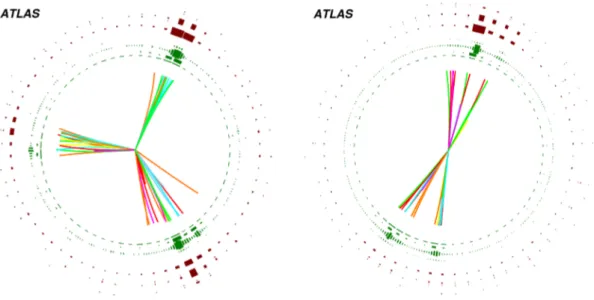
Figure 1. Transverse plane projection of a three-jet event with high values of τ⊥and S⊥ (left), and

a five-jet event with low values τ⊥ and S⊥(right). The colours are chosen for illustrative purposes.

Its eigenvalues {λ

_k

}, which satisfy

P

k

λ

k

= 1 by definition, are ordered so that λ

1

>

λ

2

> λ

3

, and the corresponding event shapes are defined as

S =

3

2

(λ

2

+ λ

3

);

A =

3

2

λ

3

.

(3.3)

S takes values between 0 and 1, with larger values indicating more spherical events.

A takes values between 0 and 1/2 and is a measure of the extent to which the radiation is

contained in the plane defined by the two first eigenvectors of the sphericity tensor defined

in eq.

3.2. The larger the value of A, the less planar the event.

The transverse linearised sphericity tensor is constructed using only the transverse

momentum components:

M

xy

=

1

P i

|~

p

i

|

X i

1

|~

p

i

|

p

2_x,i

p

x,i

p

y,i

p

y,i

p

x,i

p

2y,i

!

.

Its eigenvalues {µ

k

}, which satisfy

Pk

µ

k

= 1 by definition, are ordered so that µ

1

> µ

2

and the corresponding transverse sphericity event shape is defined as

S

⊥

=

2µ

2

µ

1

+ µ

2

.

(3.4)

It takes values between 0 and 1, with large (small) values indicating isotropic (back-to-back)

events in the transverse plane.

To illustrate the meaning of the event-shape variables, figure

1

shows two different

multijet final states. The first represents a three-jet event with large values of τ

⊥

and S

⊥

.

The second represents a five-jet event with low values of τ

⊥

and S

⊥

.

The quantities in eq.

3.3

correspond to linear combinations of the eigenvalues of the

sphericity tensor. However, one may consider quadratic and cubic combinations of the

JHEP01(2021)188

eigenvalues {λ

_i

} [26], such as

C = 3(λ

1

λ

2

+ λ

1

λ

3

+ λ

2

λ

3

),

(3.5)

D = 27(λ

1

λ

2

λ

3

).

(3.6)

The quantities defined in eqs.

3.5

and

3.6

are restricted to the range [0, 1]. These are

also useful observables to characterise multijet events. Since C is defined by products of

eigenvalue pairs, it vanishes for two-jet events, while D, which is defined by multiplying

the three eigenvalues, vanishes for events in which all jet momenta lie on the same plane.

To study the dependence of the observables on the event topology and energy scale,

each of the six event-shape observables is measured as a function of n

jet

and H

T2

. Events

that satisfy the selection requirements are classified in bins of n

jet

(= 2, 3, 4, 5 and ≥ 6)

and H

_T2

(1 TeV < H

_T2

< 1.5 TeV, 1.5 TeV < H

T2

< 2.0 TeV, H

T2

> 2 TeV).

A measurement of the multijet production cross section in the different H

_T2

bins is

performed in the same fiducial phase space in which the event-shape observables are

mea-sured, i.e. in events with 2, 3, 4, 5 or ≥ 6 jets. Since many of the experimental uncertainties

that affect the measurement of the event-shape observables are correlated between n

jet

bins,

these measurements are presented normalised to the inclusive dijet cross section in bins of

H

T2

. In this way, the experimental uncertainties discussed in section

7

are significantly

reduced while preserving important physics information, such as the relative shape of the

distributions.

4

Data and Monte Carlo samples

The dataset used in this analysis comprises the data taken from 2015 to 2018 at a

centre-of-mass energy of

√

s = 13 TeV. After applying quality criteria to ensure good ATLAS

detector operation, the total integrated luminosity useful for data analysis is 139 fb

−1

. The

average number of inelastic pp interactions produced per bunch crossing for the dataset

considered, hereafter referred to as ‘pile-up’, is hµi = 33.6.

Several MC samples were used for this analysis; they differ in the matrix element

(ME) calculation and/or the parton shower (PS). In order to populate all regions of the

spectra, these samples are divided into subsamples with differing kinematic characteristics.

The samples were produced using the Pythia [

27,

28

_{], Sherpa [}

29

_{], Herwig [}

30–32] and

MadGraph5_aMC@NLO (hereafter referred to as MG5_aMC) [

33] generators.

The Pythia sample was generated using Pythia 8.235. The matrix element (ME)

was calculated for the 2 → 2 process. The parton shower algorithm includes initial- and

final-state radiation based on the dipole-style p

T

-ordered evolution, including γ → q ¯

q

branchings and a detailed treatment of the colour connections between partons [27]. The

renormalisation and factorisation scales were set to the geometric mean of the squared

transverse masses of the two outgoing particles (labelled 3 and 4), i.e.

q

m

2_T

3

· m

2

T4

=

q

(p

2_T

+ m

2₃

) · (p

2_T

+ m

2₄

_{). The NNPDF 2.3 LO PDF set [}

34] was used in the ME

genera-tion, in the parton shower, and in the simulation of multi-parton interactions (MPI). The

ATLAS A14 [35] set of tuned parameters (tune) is used for the parton shower and MPI,

JHEP01(2021)188

whilst hadronisation was modelled using the Lund string model [36,

37

_{]. The Pythia}

sample contains per-event weights that allow the estimation of uncertainties due to the

parton shower parameters, including the variations of the renormalisation scale for QCD

initial- and final-state radiation (ISR – FSR) and variations of the non-singular terms of

the splitting functions.

The Sherpa sample was generated using Sherpa 2.1.1. The ME calculation is

in-cluded for the 2 → 2 and 2 → 3 processes at leading order (LO), and the Sherpa parton

shower [38,

39] with p

_T

ordering was used for the showering. Matrix element

renormali-sation and factorirenormali-sation scales for 2 → 2 processes were set to the harmonic mean of the

Mandelstam variables s, t and u [40], whereas the Catani-Marchesini-Webber (CMW) [41]

scale was chosen for the additional emission in 2 → 3 processes. The CT14 NNLO [

42]

PDF set was used for the matrix element calculation, while the parameters used for the

modelling of the MPI and the parton shower were set according to the CT10 tune [

43]. The

Sherpa sample makes use of the dedicated Sherpa AHADIC model for hadronisation [

44],

which is based on the cluster fragmentation algorithm [45].

The MG5_aMC+Pythia 8 sample was generated using MadGraph5_aMC@NLO

2.3.3.

The calculation includes matrix elements computed at leading order for up to

four final-state partons, using the NNPDF 3.0 NLO [

46] PDF set, and merged with the

CKKW-L prescription [47,

48]. The renormalisation and factorisation scales were set to

the transverse mass of the 2 → 2 system that results from the k

_t

clustering [49] and the

merging scale was set to 30 GeV. The parton shower and hadronisation were handled by

Pythia 8.212. The ATLAS A14 tune with the NNPDF 2.3 LO PDF set was used for the

shower and MPI, and the Lund string model was used for the modelling of hadronisation.

Finally, two Herwig samples were generated using Herwig 7.1.3 at next-to-leading

order. This includes NLO accuracy for the 2 → 2 process and LO accuracy for the 2 →

3 process. The ME was calculated using Matchbox [

50

_{] with the MMHT2014 NLO}

PDF [51]. The renormalisation and factorisation scales were set to the p

T

of the leading jet.

The first sample uses an angle-ordered parton shower, while the second sample uses a

dipole-based parton shower. In both cases, the parton shower was interfaced to the ME calculation

using the MC@NLO matching scheme. The angle-ordered shower evolves on the basis

of 1→2 splittings with massive DGLAP functions using a generalised angular variable

and employs a global recoil scheme once showering has terminated.

The dipole-based

shower uses 2→3 splittings with Catani-Seymour kernels with an ordering in transverse

momentum and so is able to perform recoils on an emission-by-emission basis. For both

Herwig samples, the parameters that control the MPI and parton shower simulation were

set according to the H7-UE-MMHT tune [

51], and the hadronisation was modelled by

means of the cluster fragmentation algorithm.

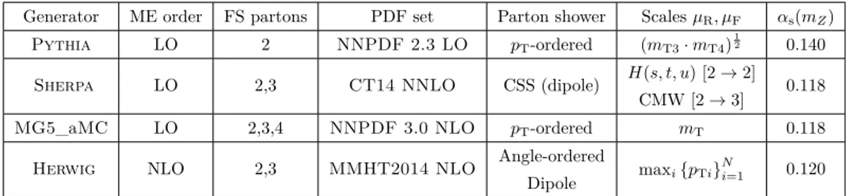
The main features of the samples described above are summarised in table

1.

The Pythia, Sherpa and Herwig samples were passed through the

Geant4-based [52] ATLAS detector-simulation program [53] since they were also used to unfold

the measurements to the particle level, as described in section

6. They are reconstructed

and analysed with the same processing chain as the data. The MG5_aMC samples are

used for comparison at particle level.

JHEP01(2021)188

Generator ME order FS partons PDF set Parton shower Scales µR, µF αs(mZ)

Pythia LO 2 NNPDF 2.3 LO pT-ordered (mT3· mT4)

1

2 0.140

Sherpa LO 2,3 CT14 NNLO CSS (dipole) H(s, t, u) [2 → 2] 0.118

CMW [2 → 3]

MG5_aMC LO 2,3,4 NNPDF 3.0 NLO pT-ordered mT 0.118

Herwig NLO 2,3 MMHT2014 NLO Angle-ordered_Dipole maxi{pTi}Ni=1 0.120

Table 1. Properties of the Monte Carlo samples used in the analysis, including the perturbative

order in αs, the number of final-state partons, the PDF set, the parton shower algorithm, the

renormalisation and factorisation scales and the value of αs(mZ) for the matrix element.

The generation of the simulated event samples includes the effect of multiple pp

inter-actions per bunch crossing, as well as the effect on the detector response of interinter-actions

from bunch crossings before or after the one containing the hard interaction. In addition,

during the data-taking, some modules (so-called “dead-tile modules”) situated in various

η-φ regions of the ATLAS hadronic calorimeter were found to be malfunctioning for some

periods of time, leading to poorly reconstructed jets in these regions. The resulting dead

re-gions in the hadronic calorimeter were included in the simulation for the Pythia, Sherpa

and Herwig samples.

5

Event selection and object reconstruction

Events with high-p

_T

jets are preselected using a single-jet trigger with a minimum p

_T

threshold of 460 GeV. Events are required to have at least one reconstructed vertex that

contains two or more associated tracks with transverse momentum p

_T

> 500 MeV. The

re-constructed vertex that maximises

P

p

2_T

, where the sum is performed over tracks associated

with the vertex, is chosen as the primary vertex.

Jets are reconstructed using the anti-k

t

algorithm [54] with radius parameter R =

0.4 using the FastJet program [

55]. The inputs to the jet algorithm are particle-flow

objects [56], which make use of both the calorimeter and the inner-detector information

to precisely determine the momenta of the input particles. The jet calibration procedure

includes energy corrections for pile-up, as well as angular corrections. Effects due to energy

losses in inactive material, shower leakage, the parameterisation of the magnetic field and

inefficiencies in energy clustering and jet reconstruction are taken into account. This is

done using a simulation-based correction, in bins of η and p

_T

, derived from the relation

of the reconstructed jet energy to the energy of the corresponding particle-level jet, not

including muons or non-interacting particles. In a final step, an in situ calibration corrects

for residual differences in the jet response between the MC simulation and the data using

p

T

-balance techniques for dijet, γ+jet, Z+jet and multijet final states.

The selected jets must have p

_T

> 100 GeV and |η| < 2.4. These requirements reject

pile-up jets and reduce experimental uncertainties. In addition, jets are required to satisfy

quality criteria that reject beam-induced backgrounds (jet cleaning) [57]. The efficiency of

this requirement for selecting good jets with p

_T

> 100 GeV is larger than 99.5%. Events

are required to have at least two selected jets. The two leading jets are further required

JHEP01(2021)188

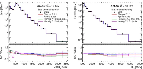
] -1 Jets [GeV 1 10 2 10 3 10 4 10 5 10 ATLAS s = 13 TeV

Stat. uncertainty only Data Sherpa 2.1.1 Pythia 8.235 Herwig 7.1.3 ang. ord. Herwig 7.1.3 dipole [GeV] T Jet p 500 1000 1500 2000 2500 3000 3500 MC / Data 0.8 1 1.2 ] -1 Events [GeV -1 10 1 10 2 10 3 10 4 10 5 10 ATLAS _{s = 13 TeV}

Stat. uncertainty only Data Sherpa 2.1.1 Pythia 8.235 Herwig 7.1.3 ang. ord. Herwig 7.1.3 dipole [GeV] T2 H 1000 2000 3000 4000 5000 6000 7000 MC / Data 0.8 1 1.2

Figure 2. Detector level distributions of the transverse momenta of all jets (left) and the scalar

sum of transverse momenta of the two leading jets (right), together with MC predictions. Only statistical uncertainties are shown.

to satisfy H

_T2

> 1 TeV. This requirement ensures a trigger efficiency of ≈100%. About

57.5 million events in data satisfy the selection criteria.

Figure

2

shows the detector

level distributions for the selected jets p

_T

and H

_T2

, along with MC predictions.

The

binning of the event-shape distributions is chosen as a compromise between maximising

the number of bins while minimising migration between bins due to the resolution of the

measured variables.

6

Unfolding to particle level

In order to make meaningful comparisons with particle-level MC predictions, the

event-shape distributions need to be corrected for distortions induced by the response of the

ATLAS detector and associated reconstruction algorithms. The fiducial phase-space region

is defined at particle level for all particles with a mean decay length cτ > 10 mm; these

particles are referred to as ‘stable’. Particle-level jets are reconstructed using the anti-k

_t

algorithm with R = 0.4 using stable particles, excluding muons and neutrinos. The fiducial

phase space closely follows the event selection criteria defined in section

5. Particle-level

jets are required to have p

_T

> 100 GeV and |y| < 2.4, where y represents the rapidity.

Events with at least two particle-level jets are considered. These events are also required

to have H

_T2

> 1 TeV.

The unfolding is performed using an iterative algorithm based on Bayes’ theorem [58].

The algorithm takes into account inefficiencies and resolution effects due to the detector

response that lead to bin migrations between the detector-level and particle-level phase

spaces. For each observable, the method makes use of a transfer matrix, M

_ij

, obtained

from MC simulation, that parameterises the probability of an event generated in bin i to

be reconstructed in bin j. The correction can thus be written as a linear equation

N

JHEP01(2021)188

The quantities R

_i

and T

_j

are the contents of the detector-level distribution in bin i

and the contents of the particle-level distribution in bin j, respectively, while the factors

E

_j

and P

_i

are the efficiency and the purity, which are estimated using the MC simulation.

Migrations between detector- and particle-level phase spaces due to different values of n

jet

and H

_T2

are taken into account in the unfolding procedure for event-shape observables. Due

to the fine binning of the measured distributions, detector resolution is the primary cause of

bin migrations between detector- and particle-level phase spaces, followed by the jet energy

resolution, which leads to different values of n

jet

between the detector and particle levels.

The efficiency E

_j

is used to correct for events in the particle-level phase space which are

not reconstructed at detector level. The binned efficiency is defined by the number of MC

events that satisfy all the selection requirements at both the detector and particle levels

and are generated and reconstructed in the same event-shape bin, with the same n

jet

and

H

T2

range, divided by the number of events generated in the same event-shape, n

jet

and

H

T2

bin. For low values of the event-shape variables the efficiency is typically close to 80%,

while for large values it decreases to ≈ 40%. In addition, the binned efficiency tends to have

lower values at higher n

jet

for the same event-shape bin. The purity P

i

is used to correct

for events in the detector-level phase space that do not have a particle-level counterpart.

The binned purity is defined as the number of events that satisfy selection requirements at

particle and detector levels divided by those reconstructed in the same event-shape, n

jet

and

H

T2

bin. Similarly to the bin-by-bin efficiency, the purity is close to 80% for low values of

the event-shape variables and decreases to 40–50% for large values. The bin-by-bin purity

tends to have lower values for the same event-shape bin at higher n

jet

. Since the bin-by-bin

purity and efficiency distributions are similar, and the migrations in the transfer matrices

are mainly between neighbouring bins of the event-shape distributions, the impact of the

unfolding on the shape of the distributions is modest. The results obtained by unfolding

the data with Pythia are used to obtain the nominal differential cross sections, whereas

Sherpa and Herwig MC predictions are used to estimate the systematic uncertainty due

to the model dependence, as discussed in section

7.

7

Experimental uncertainties

The dominant sources of systematic uncertainty in the measurements arise from imperfect

knowledge of the jet energy scale and resolution and the modelling of the strong interaction.

The systematic uncertainties are propagated through the unfolding via their impact on the

transfer matrices. The inclusive cross section for events with at least two jets is recomputed

for each systematic variation and used consistently in the analysis. As an example, the

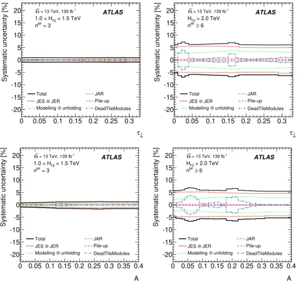
breakdown of the relative systematic uncertainties in the measurement of the normalised

differential cross sections as functions of τ

⊥

and A is shown in figure

3.

A detailed description of the systematic uncertainties and their values for normalised

event-shape observables is given below:

• Jet Energy Scale and Resolution: the jet energy scale (JES) and jet energy resolution

(JER) uncertainties are estimated as described in ref. [59]. The JES is calibrated on

the basis of the simulation, including in situ corrections obtained from data. The

JHEP01(2021)188

τ 0 0.05 0.1 0.15 0.2 0.25 0.3 Systematic uncertainty [%] -20 -15 -10 -5 0 5 10 15 20 Total JER ⊕ JES unfolding ⊕ Modelling JAR Pile-up DeadTileModules < 1.5 TeV T2 1.0 < H = 3 jet n ATLAS -1 = 13 TeV, 139 fb s τ 0 0.05 0.1 0.15 0.2 0.25 0.3 Systematic uncertainty [%] -20 -15 -10 -5 0 5 10 15 20 Total JER ⊕ JES unfolding ⊕ Modelling JAR Pile-up DeadTileModules > 2.0 TeV T2 H 6 ≥ jet n ATLAS -1 = 13 TeV, 139 fb s A 0 0.05 0.1 0.15 0.2 0.25 0.3 0.35 0.4 Systematic uncertainty [%] -20 -15 -10 -5 0 5 10 15 20 Total JER ⊕ JES unfolding ⊕ Modelling JAR Pile-up DeadTileModules < 1.5 TeV T2 1.0 < H = 3 jet n ATLAS -1 = 13 TeV, 139 fb s A 0 0.05 0.1 0.15 0.2 0.25 0.3 0.35 0.4 Systematic uncertainty [%] -20 -15 -10 -5 0 5 10 15 20 Total JER ⊕ JES unfolding ⊕ Modelling JAR Pile-up DeadTileModules > 2.0 TeV T2 H 6 ≥ jet n ATLAS -1 = 13 TeV, 139 fb s

Figure 3. Breakdown of the systematic uncertainties as a function of τ⊥(top) and A (bottom) for

selected regions of HT2 and njet.

JES uncertainties are estimated using a decorrelation scheme comprising a set of

44 independent components, which depend on the jet p

T

and η.

The total JES

uncertainty in the p

_T

value of individual jets is < 2% at p

_T

= 100 GeV with a mild

dependence on η. The JER uncertainty is estimated using a decorrelation scheme

involving 26 independent components. The effect of the total JER uncertainty is

evaluated by smearing the energy of the jets in the MC simulation by about 1.5% at

p

T

= 100 GeV to about 0.5% for p

T

of several hundred GeV. In this measurement,

the JES and JER uncertainties are propagated by varying the energy and p

_T

of each

jet by one standard deviation of each of the independent components. The total

uncertainty in the normalised event-shape distributions varies from 1% in the lowest

n

jet

bins to 7% for the highest n

jet

, while it ranges from 7% to 14% on the fiducial

cross sections. This is the dominant source of uncertainty for high n

jet

_.

JHEP01(2021)188

• Jet Angular Resolution: the jet angular resolution (JAR) uncertainty is estimated

conservatively by smearing the angular coordinates (η, φ) of the jets by the resolution

in MC simulation. The η and φ variations are done with the p

_T

component of the jets

held constant. The value of the JAR uncertainty is below 0.5% for the normalised

event-shape distributions in all regions of the phase space, while it ranges from 1%

to 2% for the fiducial cross sections, as n

jet

increases.

• Pile-up: the uncertainty from pile-up is evaluated by varying the pile-up reweighting

procedure (see section

4) to cover the difference between the predicted inelastic cross

section and the measured value [60]. The impact of this uncertainty is below 0.5% in

all regions of the phase space, for both the event-shape and fiducial cross-section

mea-surements. As a cross-check, the event-shape distributions were compared in different

slices of hµi and between different data-taking periods, yielding compatible results.

• Unfolding: the mismodelling of the data in the MC simulation is accounted for as

an additional source of uncertainty. This is assessed by reweighting the particle-level

distributions so that the detector-level event shapes predicted by the MC samples

match those in the data. The modified detector-level distributions are then unfolded

using the method described in section

6. The difference between the modified

particle-level distribution and the nominal one is taken as the uncertainty. This uncertainty

ranges from 0.2% to a few per cent with increasing n

jet

, depending on the observable

under study.

• Modelling: the modelling uncertainty is estimated by comparing the unfolded

dis-tributions using Pythia, Sherpa and Herwig. In order to not double count the

effect of having different priors in the unfolding procedure (the so-called unfolding

uncertainty), Pythia, Sherpa and Herwig MC predictions are weighted to describe

the data. These weighted MC samples are then used to perform the unfolding and

the envelope of the differences between the estimated cross sections defines the

sys-tematic uncertainty. The value of this uncertainty for the normalised event-shape

measurement increases with n

jet

and H

T2

and varies between 1% and 4–5%,

depend-ing on the observable under study. For the fiducial cross-section measurement this

uncertainty is below 5%.

• Luminosity: the uncertainty in the combined 2015–2018 integrated luminosity is

1.7% [61], obtained using the LUCID-2 detector [62] for the primary luminosity

mea-surements.

The measurements of event-shape observables are unaffected by this

uncertainty, given that they are normalised to the inclusive dijet cross section, thus

cancelling out the contribution of the luminosity.

• Dead-tile modules: a systematic uncertainty is derived to address the possible bias

on the measurements due to the residual mismodeling of disabled portions of the tile

calorimeter by the MC simulations. New differential cross-sections are derived by

vetoing events in data and MC simulation where at least one of these non-operating

modules is found within the selected jets. The difference between this result and the

nominal one is taken as the uncertainty. The value of this uncertainty is below 1%

JHEP01(2021)188

in most regions of the phase space, although it can reach values up to 4% in some

regions for the highest jet multiplicity bin.

The total systematic uncertainty is estimated by adding in quadrature the effects

previously listed. In addition, the statistical uncertainty of the data and MC simulation is

propagated to the differential cross sections through the unfolding procedure using

pseudo-experiments in order to properly take into account the statistical correlations between

bins of the event-shape variables, n

jet

and H

_T2

ranges. Moreover, the pseudo-experiments

are also used to estimate the statistical component of each systematic uncertainty. This

statistical component is reduced using the Gaussian Kernel smoothing technique [63]. The

values provided above are quoted after application of this procedure.

In general the modelling uncertainty tends to dominate at low values of n

jet

while, at

high n

jet

, the JES uncertainty dominates. The total systematic uncertainty is typically

constant for the measured differential cross sections, but increases as a function of n

jet

from ∼1% to ∼6%. For the fiducial cross sections, the uncertainties increase from ∼5% to

∼9% as a function of n

jet

_.

8

Results

The differential cross-section measurements are presented and compared with the MC

predictions described in section

4. The cross section as a function of n

jet

is shown in figure

4,

while unfolded and normalised event-shape distributions are shown in figures

5–10. The

full set of observables is presented in each H

T2

and n

jet

bin in which the measurement is

performed. The ratio of the MC prediction to the yield in data in each bin is also shown.

Figure

4

shows the fiducial cross section as a function of n

jet

in different H

_T2

ranges.

The fiducial cross section is measured in the same phase-space regions as the

differen-tial measurements. The MC predictions are normalised to the measured integrated cross

section in each H

_T2

range to compare the shape of these predictions to the data. The

normalisation factors for Herwig based on angle-ordered showers and Sherpa predictions

increase as a function of H

T2

, whereas a very small dependence of these factors on H

T2

is observed for Herwig 7 based on dipole showers, MG5_aMC and Pythia predictions.

The normalisation factors for LO accuracy MC predictions such as Pythia, MG5_aMC

and Sherpa are expected to strongly depend on the MC tune. In particular, the Pythia

prediction overestimates the inclusive dijet production cross section in the studied

phase-space region by 30%, which can be attributed to the large value of α

S

included in the

Pythia tune (see table

1

), whereas the MG5_aMC prediction underestimates it by 35%.

The Sherpa prediction gives an adequate description of the measured integrated cross

sections. In addition, an excellent description of the inclusive dijet production cross

sec-tion is found for the Herwig 7 predicsec-tion based on dipole showers, whereas Herwig 7

prediction based on angle-ordered showers underestimates it, at most by 9%. The Pythia

prediction provides a good description of the shape of the differential cross section as a

function of n

jet

_{. The Herwig 7 prediction based on angle-ordered showers gives a good}

description of the fiducial cross sections as a function of n

jet

_{. Sherpa tends to overestimate}

JHEP01(2021)188

the cross sections for n

jet

_{> 4. The Herwig 7 based on dipole showers and MG5_aMC}

predictions, while giving a good description of the cross section at low n

jet

, underestimate

the measurements at high n

jet

.

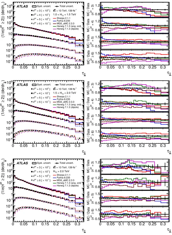
Figure

5

shows the normalised cross section as a function of τ

⊥

. For low n

jet

, the

MC simulations tend to underestimate the measurement in the intermediate region of

τ

⊥

, with the exception of the Herwig 7 predictions. At high values of τ

⊥

, where the

population of isotropic events is expected to be larger, all MC predictions underestimate

the measurements. In particular, the largest deviation is found for the Pythia prediction

where the high-p

_T

third jet is less likely to be produced isotropically. The shape of the

distributions tends to agree with data for larger n

jet

_{. Pythia tends to overestimate the}

measurements at low values of τ

⊥

, whereas the Herwig 7 prediction based on dipole

showers highly underestimates the measurements in such region. The behaviour of τ

⊥

as a

function of H

T2

indicates more isotropic events at low energies, with increasing alignment

of jets with the thrust axis for higher energy scales. Figure

6

shows the normalised cross

section as a function of T

_m

, with very similar conclusions.

Figure

7

shows the normalised cross section as a function of S

⊥

. In line with the

observations for τ

⊥

and T

m

, the results show that, for low n

jet

, Pythia and Sherpa

sim-ulations predict fewer isotropic events than in data, while the Herwig 7 and MG5_aMC

predictions are closer to the measurements. In addition, while Pythia gives an adequate

description in the intermediate region of S

⊥

, it overestimates the measurements at low

S

⊥

. For larger n

jet

, the description of the shape is improved in MC simulations, while a

discrepancy in the normalisation is observed for different predictions.

Figure

8

_{shows the normalised cross section as a function of A. In this case, the Herwig}

7 prediction with angle-ordered parton shower aligns with the rest of the MC simulations,

predicting more planar events than data at low n

jet

_{, while the Herwig 7 prediction with}

the dipole parton shower predicts higher cross sections at high A for low n

jet

.

The normalised cross sections for the quadratic observable C are shown in figure

9.

Here, larger spreads are shown in the lower tails of the distributions for low n

jet

_{. Pythia}

and Herwig 7 with the dipole-based parton shower predict a smaller cross section than

data in these regions, while the other MC predictions overestimate the measurements.

As with other event-shape observables, a larger spread is found in the normalisations at

high n

jet

_.

The cubic observable D is presented in figure

10, with conclusions similar to those

for A. The Herwig 7 prediction with dipole-based parton shower predicts a higher cross

section than data at high values of D for low n

jet

, while the other MC predictions have

the opposite behaviour. For higher n

jet

, the description of the shape becomes more similar

among different MC predictions, with differences observed in the normalisation of the

measurements.

Theoretical uncertainties on the MC predictions are not included in the discussion

of the results, since the ME for the current predictions has leading order accuracy in

the description of inclusive three-jet cross sections. This makes the usual variations of

the renormalisation and factorisation scales not reliable for the estimation of theoretical

uncertainties. To identify the phase-space regions of the event-shape variables which are

JHEP01(2021)188

more sensitive to the MC tune, variations of the parton shower parameters were examined in

Pythia as detailed in section

4. The effect of these variations on event-shape observables

typically increases with jet multiplicity. Varying the FSR energy-scale parameter by a

factor of two leads to differences of up to 40% at high values of the event-shape variables

i.e regions where the contribution of isotropic events is larger. On the other hand, varying

the ISR energy-scale parameter typically leads to differences from 10 to 30% at low values

of the event shapes for high jet multiplicities. Finally, varying the non-singular terms of the

splitting functions contributes a 5–10% difference that is typically constant as a function

of the event-shape variables.

In summary, none of the MC predictions investigated provide a good description of

the data in all regions of the phase space. In general, at low n

jet

_{, Pythia and Sherpa}

predictions underestimate the measurements at high values of the event-shape distributions,

i.e. events in data follow a more isotropic distribution of the energy flow than those from

these two predictions. Pythia shows discrepancies of up to 80%. This shows the limited

ability of parton shower models to simulate hard and wide angle radiation. The addition of

2 → 3 processes in the ME allows to improve the description of the measurements in such

regions. While Sherpa can differ by up to 30%, the Herwig and MG5_aMC predictions

show discrepancies of 10-20%. Moreover, both Herwig 7 predictions overestimate the

central regions of τ

⊥

by up to 20%, while differing in the description of the aplanarity: the

angle-ordered parton shower gives rise to more planar events than in data, while the

dipole-based parton shower overestimates the measurements at high values of A for n

jet

= 3. In

addition, the Herwig 7 prediction with dipole-based parton shower underestimates the

measurements at low values of the event-shape distributions, whereas the Herwig 7

angle-ordered prediction gives a better description in these regions. Overall, the description of the

measurements made by the Herwig 7 prediction based on angle-ordered parton showers is

better than the description by the dipole-based parton shower. This may be due to the fact

that the Herwig 7 dipole-based shower model is recently released, and the parameters have

not been tuned as thoroughly as those of the more mature angle-ordered showers. Moreover,

the MG5_aMC prediction which includes up to four final-state partons in the ME gives

the best overall description of the shape of the measurements in the studied n

jet

and H

T2

bins. This shows the importance of including in the ME beyond LO terms to describe the

dynamics of high-p

_T

multijet final states. At high n

jet

_{, all MC simulations tend to give}

a similar prediction for the shape of the distributions. However, the normalisation of the

predictions shows a large spread between different MC simulations in each bin of the jet

multiplicity. The Sherpa prediction gives an adequate description of the normalisation

for n

jet

≤ 4, although it overestimates the cross sections up to 30% for high n

jet

_{. The}

MG5_aMC and the Herwig 7 with dipole-based parton showers simulations predict

cross sections up to 30% lower for events with at least six jets. Finally, Herwig 7 with

angle-ordered parton shower and Pythia predictions give a reasonably good description

of the normalisation of the differential cross sections for the studied jet multiplicity and

H

T2

bins.

All measurements can be found in Hepdata [

64], including these measurements binned

in inclusive jet multiplicity.

JHEP01(2021)188

jet n 2 3 4 5 ≥ 6 [pb] jet /dn σ d 1 10 2 10 1.01) × Sherpa 2.1.1 ( 0.71) × Pythia 8.235 ( 1.36) × MG5_aMC 2.3.3 ( 1.03) ×

Herwig 7.1.3 ang. ord ( 1.00) × Herwig 7.1.3 dipole ( ATLAS -1 = 13 TeV, 139 fb s 1.0 < HT2 < 1.5 TeV

Syst. uncert. Total uncert.

MC / Data 0.5 1 1.5 MC / Data _0.5 1 1.5 MC / Data _0.5 1 1.5 jet

n

2 3 4 5 ≥ 6 MC / Data 0.5 1 1.5 jet n 2 3 4 5 ≥ 6 [pb] jet /dn σ d -1 10 1 10 1.04) × Sherpa 2.1.1 ( 0.70) × Pythia 8.235 ( 1.37) × MG5_aMC 2.3.3 ( 1.07) ×

Herwig 7.1.3 ang. ord ( 0.99) × Herwig 7.1.3 dipole ( ATLAS -1 = 13 TeV, 139 fb s 1.5 < H_T2 < 2.0 TeV

Syst. uncert. Total uncert.

MC / Data 0.5 1 1.5 MC / Data _0.5 1 1.5 MC / Data _0.5 1 1.5 jet

n

2 3 4 5 ≥ 6 MC / Data 0.5 1 1.5 jet n 2 3 4 5 ≥ 6 [pb] jet /dn σ d -1 10 1 10 1.06) × Sherpa 2.1.1 ( 0.70) × Pythia 8.235 ( 1.37) × MG5_aMC 2.3.3 ( 1.09) ×

Herwig 7.1.3 ang. ord ( 1.00) × Herwig 7.1.3 dipole ( ATLAS -1 = 13 TeV, 139 fb s HT2 > 2.0 TeV

Syst. uncert. Total uncert.

MC / Data 0.5 1 1.5 MC / Data _0.5 1 1.5 MC / Data _0.5 1 1.5 jet

n

2 3 4 5 ≥ 6 MC / Data 0.5 1 1.5

Figure 4. Fiducial cross section as a function of jet multiplicity. The MC predictions are normalised

to the measured integrated cross section for njet ≥ 2 in each HT2 bin using the factors indicated

in parentheses. The right panels show the ratios of the MC distributions to the data distributions. The error bars show the total uncertainty (statistical and systematic added in quadrature) and the grey bands in the right panels show the systematic uncertainty.

JHEP01(2021)188

τ 0 0.05 0.1 0.15 0.2 0.25 0.3 ) τ /d σ 2)) (d ≥ jet (n σ (1/ -4 10 -3 10 -2 10 -1 10 1 10 2 10 3 10 4 10 5 10 6 10 Sherpa 2.1.1 Pythia 8.235 MG5_aMC 2.3.3 Herwig 7.1.3 (ang. ord) Herwig 7.1.3 (dipole) ] 2 10 × = 3 [ jet n ] 1 10 × = 4 [ jet n ] 0 10 × = 5 [ jet n ] -1 10 × 6 [ ≥ jet n ATLAS -1 = 13 TeV, 139 fb s < 1.5 TeV T2 1.0 < H Syst. uncert. Total uncert.

= 3) jet (n MC / Data 0.8 1 1.2 = 4) jet (n MC / Data 0.8 1 1.2 = 5) jet (n MC / Data 0.5 1 1.5 τ 0 0.05 0.1 0.15 0.2 0.25 0.3 ) 6 ≥ jet (n MC / Data 0.5 1 1.5 τ 0 0.05 0.1 0.15 0.2 0.25 0.3 ) τ /d σ 2)) (d ≥ jet (n σ (1/ -4 10 -3 10 -2 10 -1 10 1 10 2 10 3 10 4 10 5 10 6 10 Sherpa 2.1.1 Pythia 8.235 MG5_aMC 2.3.3 Herwig 7.1.3 (ang. ord) Herwig 7.1.3 (dipole) ] 2 10 × = 3 [ jet n ] 1 10 × = 4 [ jet n ] 0 10 × = 5 [ jet n ] -1 10 × 6 [ ≥ jet n ATLAS -1 = 13 TeV, 139 fb s < 2.0 TeV T2 1.5 < H Syst. uncert. Total uncert.

= 3) jet (n MC / Data 0.8 1 1.2 = 4) jet (n MC / Data 0.8 1 1.2 = 5) jet (n MC / Data 0.5 1 1.5 τ 0 0.05 0.1 0.15 0.2 0.25 0.3 ) 6 ≥ jet (n MC / Data 0.5 1 1.5 τ 0 0.05 0.1 0.15 0.2 0.25 0.3 ) τ /d σ 2)) (d ≥ jet (n σ (1/ -4 10 -3 10 -2 10 -1 10 1 10 2 10 3 10 4 10 5 10 Sherpa 2.1.1 Pythia 8.235 MG5_aMC 2.3.3 Herwig 7.1.3 (ang. ord) Herwig 7.1.3 (dipole) ] 2 10 × = 3 [ jet n ] 1 10 × = 4 [ jet n ] 0 10 × = 5 [ jet n ] -1 10 × 6 [ ≥ jet n ATLAS -1 = 13 TeV, 139 fb s > 2.0 TeV T2 H

Syst. uncert. Total uncert.

= 3) jet (n MC / Data 0.8 1 1.2 = 4) jet (n MC / Data 0.8 1 1.2 = 5) jet (n MC / Data 0.5 1 1.5 τ 0 0.05 0.1 0.15 0.2 0.25 0.3 ) 6 ≥ jet (n MC / Data 0.5 1 1.5

Figure 5. Comparison between data and MC simulation as a function of the transverse thrust

τ⊥ (see eq. 3.1) for different jet multiplicities and energy scales. For illustration purposes, the

corresponding differential cross section for each jet multiplicity is multiplied by 102_(njet_{= 3), 10}1

(njet_{= 4), 10}0 _(njet_{= 5), 10}−1 _(njet_{≥ 6). The right panels show the ratios between the MC and}

the data distributions. The error bars show the total uncertainty (statistical and systematic added in quadrature) and the grey bands in the right panels show the systematic uncertainty.

JHEP01(2021)188

m T 0 0.1 0.2 0.3 0.4 0.5 0.6 ) m /dT σ 2)) (d ≥ jet (n σ (1/ -6 10 -5 10 -4 10 -3 10 -2 10 -1 10 1 10 2 10 3 10 4 10 5 10 6 10 7 10 Sherpa 2.1.1 Pythia 8.235 MG5_aMC 2.3.3 Herwig 7.1.3 (ang. ord) Herwig 7.1.3 (dipole) ] 2 10 × = 3 [ jet n ] 1 10 × = 4 [ jet n ] 0 10 × = 5 [ jet n ] -1 10 × 6 [ ≥ jet n ATLAS -1 = 13 TeV, 139 fb s < 1.5 TeV T2 1.0 < H

Syst. uncert. Total uncert.

= 3) jet (n MC / Data 0.8 1 1.2 = 4) jet (n MC / Data 0.8 1 1.2 = 5) jet (n MC / Data 0.5 1 1.5 m

T

0 0.1 0.2 0.3 0.4 0.5 0.6 ) 6 ≥ jet (n MC / Data 0.5 1 1.5 m T 0 0.1 0.2 0.3 0.4 0.5 0.6 ) m /dT σ 2)) (d ≥ jet (n σ (1/ -6 10 -5 10 -4 10 -3 10 -2 10 -1 10 1 10 2 10 3 10 4 10 5 10 6 10 7 10 Sherpa 2.1.1 Pythia 8.235 MG5_aMC 2.3.3 Herwig 7.1.3 (ang. ord) Herwig 7.1.3 (dipole) ] 2 10 × = 3 [ jet n ] 1 10 × = 4 [ jet n ] 0 10 × = 5 [ jet n ] -1 10 × 6 [ ≥ jet n ATLAS -1 = 13 TeV, 139 fb s < 2.0 TeV T2 1.5 < H

Syst. uncert. Total uncert.

= 3) jet (n MC / Data 0.8 1 1.2 = 4) jet (n MC / Data 0.8 1 1.2 = 5) jet (n MC / Data 0.5 1 1.5 m

T

0 0.1 0.2 0.3 0.4 0.5 0.6 ) 6 ≥ jet (n MC / Data 0.5 1 1.5 m T 0 0.1 0.2 0.3 0.4 0.5 0.6 ) m /dT σ 2)) (d ≥ jet (n σ (1/ -5 10 -4 10 -3 10 -2 10 -1 10 1 10 2 10 3 10 4 10 5 10 6 10 Sherpa 2.1.1 Pythia 8.235 MG5_aMC 2.3.3 Herwig 7.1.3 (ang. ord) Herwig 7.1.3 (dipole) ] 2 10 × = 3 [ jet n ] 1 10 × = 4 [ jet n ] 0 10 × = 5 [ jet n ] -1 10 × 6 [ ≥ jet n ATLAS -1 = 13 TeV, 139 fb s > 2.0 TeV T2 H

Syst. uncert. Total uncert.

= 3) jet (n MC / Data 0.8 1 1.2 = 4) jet (n MC / Data 0.8 1 1.2 = 5) jet (n MC / Data 0.5 1 1.5 m

T

0 0.1 0.2 0.3 0.4 0.5 0.6 ) 6 ≥ jet (n MC / Data 0.5 1 1.5

Figure 6. Comparison between data and MC predictions as a function of the transverse minor

Tm (see eq. 3.1) for different jet multiplicities and energy scales. For illustration purposes, the

corresponding differential cross section for each jet multiplicity is multiplied by 102_(njet_{= 3), 10}1

(njet_{= 4), 10}0 _(njet_{= 5), 10}−1 _(njet_{≥ 6). The right panels show the ratios between the MC and}

the data distributions. The error bars show the total uncertainty (statistical and systematic added in quadrature) and the grey bands in the right panels show the systematic uncertainty.

JHEP01(2021)188

S 0 0.1 0.2 0.3 0.4 0.5 0.6 0.7 0.8 0.9 1 ) /dS σ 2)) (d ≥ jet (n σ (1/ -6 10 -5 10 -4 10 -3 10 -2 10 -1 10 1 10 2 10 3 10 4 10 5 10 6 10 Sherpa 2.1.1 Pythia 8.235 MG5_aMC 2.3.3 Herwig 7.1.3 (ang. ord) Herwig 7.1.3 (dipole) ] 2 10 × = 3 [ jet n ] 1 10 × = 4 [ jet n ] 0 10 × = 5 [ jet n ] -1 10 × 6 [ ≥ jet n ATLAS -1 = 13 TeV, 139 fb s < 1.5 TeV T2 1.0 < H Syst. uncert. Total uncert.

= 3) jet (n MC / Data 0.8 1 1.2 = 4) jet (n MC / Data 0.8 1 1.2 = 5) jet (n MC / Data 0.5 1 1.5 S 0 0.1 0.2 0.3 0.4 0.5 0.6 0.7 0.8 0.9 1 ) 6 ≥ jet (n MC / Data 0.5 1 1.5 S 0 0.1 0.2 0.3 0.4 0.5 0.6 0.7 0.8 0.9 1 ) /dS σ 2)) (d ≥ jet (n σ (1/ -6 10 -5 10 -4 10 -3 10 -2 10 -1 10 1 10 2 10 3 10 4 10 5 10 6 10 Sherpa 2.1.1 Pythia 8.235 MG5_aMC 2.3.3 Herwig 7.1.3 (ang. ord) Herwig 7.1.3 (dipole) ] 2 10 × = 3 [ jet n ] 1 10 × = 4 [ jet n ] 0 10 × = 5 [ jet n ] -1 10 × 6 [ ≥ jet n ATLAS -1 = 13 TeV, 139 fb s < 2.0 TeV T2 1.5 < H Syst. uncert. Total uncert.

= 3) jet (n MC / Data 0.8 1 1.2 = 4) jet (n MC / Data 0.8 1 1.2 = 5) jet (n MC / Data 0.5 1 1.5 S 0 0.1 0.2 0.3 0.4 0.5 0.6 0.7 0.8 0.9 1 ) 6 ≥ jet (n MC / Data 0.5 1 1.5 S 0 0.1 0.2 0.3 0.4 0.5 0.6 0.7 0.8 0.9 1 ) /dS σ 2)) (d ≥ jet (n σ (1/ -6 10 -5 10 -4 10 -3 10 -2 10 -1 10 1 10 2 10 3 10 4 10 5 10 6 10 Sherpa 2.1.1 Pythia 8.235 MG5_aMC 2.3.3 Herwig 7.1.3 (ang. ord) Herwig 7.1.3 (dipole) ] 2 10 × = 3 [ jet n ] 1 10 × = 4 [ jet n ] 0 10 × = 5 [ jet n ] -1 10 × 6 [ ≥ jet n ATLAS -1 = 13 TeV, 139 fb s > 2.0 TeV T2 H

Syst. uncert. Total uncert.

= 3) jet (n MC / Data 0.8 1 1.2 = 4) jet (n MC / Data 0.8 1 1.2 = 5) jet (n MC / Data 0.5 1 1.5 S 0 0.1 0.2 0.3 0.4 0.5 0.6 0.7 0.8 0.9 1 ) 6 ≥ jet (n MC / Data 0.5 1 1.5

Figure 7. Comparison between data and MC predictions as a function of the transverse sphericity

S⊥ (see eq. 3.4) for different jet multiplicities and energy scales. For illustration purposes, the

corresponding differential cross section for each jet multiplicity is multiplied by 102_(njet_{= 3), 10}1

(njet_{= 4), 10}0 _(njet_{= 5), 10}−1 _(njet_{≥ 6). The right panels show the ratios between the MC and}

the data distributions. The error bars show the total uncertainty (statistical and systematic added in quadrature) and the grey bands in the right panels show the systematic uncertainty.

JHEP01(2021)188

A 0 0.05 0.1 0.15 0.2 0.25 0.3 0.35 0.4 /dA) σ 2)) (d ≥ jet (n σ (1/ -5 10 -4 10 -3 10 -2 10 -1 10 1 10 2 10 3 10 4 10 5 10 6 10 Sherpa 2.1.1 Pythia 8.235 MG5_aMC 2.3.3 Herwig 7.1.3 (ang. ord) Herwig 7.1.3 (dipole) ] 2 10 × = 3 [ jet n ] 1 10 × = 4 [ jet n ] 0 10 × = 5 [ jet n ] -1 10 × 6 [ ≥ jet n ATLAS -1 = 13 TeV, 139 fb s < 1.5 TeV T2 1.0 < H

Syst. uncert. Total uncert.

= 3) jet (n MC / Data 0.8 1 1.2 = 4) jet (n MC / Data 0.8 1 1.2 = 5) jet (n MC / Data 0.5 1 1.5

A

0 0.05 0.1 0.15 0.2 0.25 0.3 0.35 0.4 ) 6 ≥ jet (n MC / Data 0.5 1 1.5 A 0 0.05 0.1 0.15 0.2 0.25 0.3 0.35 0.4 /dA) σ 2)) (d ≥ jet (n σ (1/ -5 10 -4 10 -3 10 -2 10 -1 10 1 10 2 10 3 10 4 10 5 10 Sherpa 2.1.1 Pythia 8.235 MG5_aMC 2.3.3 Herwig 7.1.3 (ang. ord) Herwig 7.1.3 (dipole) ] 2 10 × = 3 [ jet n ] 1 10 × = 4 [ jet n ] 0 10 × = 5 [ jet n ] -1 10 × 6 [ ≥ jet n ATLAS -1 = 13 TeV, 139 fb s < 2.0 TeV T2 1.5 < H

Syst. uncert. Total uncert.

= 3) jet (n MC / Data 0.8 1 1.2 = 4) jet (n MC / Data 0.8 1 1.2 = 5) jet (n MC / Data 0.5 1 1.5

A

0 0.05 0.1 0.15 0.2 0.25 0.3 0.35 0.4 ) 6 ≥ jet (n MC / Data 0.5 1 1.5 A 0 0.05 0.1 0.15 0.2 0.25 0.3 0.35 0.4 /dA) σ 2)) (d ≥ jet (n σ (1/ -5 10 -4 10 -3 10 -2 10 -1 10 1 10 2 10 3 10 4 10 5 10 Sherpa 2.1.1 Pythia 8.235 MG5_aMC 2.3.3 Herwig 7.1.3 (ang. ord) Herwig 7.1.3 (dipole) ] 2 10 × = 3 [ jet n ] 1 10 × = 4 [ jet n ] 0 10 × = 5 [ jet n ] -1 10 × 6 [ ≥ jet n ATLAS -1 = 13 TeV, 139 fb s > 2.0 TeV T2 H

Syst. uncert. Total uncert.

= 3) jet (n MC / Data 0.8 1 1.2 = 4) jet (n MC / Data 0.8 1 1.2 = 5) jet (n MC / Data 0.5 1 1.5

A

0 0.05 0.1 0.15 0.2 0.25 0.3 0.35 0.4 ) 6 ≥ jet (n MC / Data 0.5 1 1.5

Figure 8. Comparison between data and MC predictions as a function of the aplanarity A (see

eq.3.3) for different jet multiplicities and energy scales. For illustration purposes, the correspond-ing differential cross section for each jet multiplicity is multiplied by 102 _(njet _{= 3), 10}1 _(njet ₌

4), 100 _(njet _{= 5), 10}−1 _(njet _{≥ 6). The right panels show the ratios between the MC and the}

data distributions. The error bars show the total uncertainty (statistical and systematic added in quadrature) and the grey bands in the right panels show the systematic uncertainty.

JHEP01(2021)188

C 0 0.1 0.2 0.3 0.4 0.5 0.6 0.7 0.8 0.9 1 /dC) σ 2)) (d ≥ jet (n σ (1/ -7 10 -6 10 -5 10 -4 10 -3 10 -2 10 -1 101 10 2 10 3 10 4 10 5 10 6 10 7 10 8 10 9 10 Sherpa 2.1.1 Pythia 8.235 MG5_aMC 2.3.3 Herwig 7.1.3 (ang. ord) Herwig 7.1.3 (dipole) ] 2 10 × = 3 [ jet n ] 1 10 × = 4 [ jet n ] 0 10 × = 5 [ jet n ] -1 10 × 6 [ ≥ jet n ATLAS -1 = 13 TeV, 139 fb s < 1.5 TeV T2 1.0 < H

Syst. uncert. Total uncert.

= 3) jet (n MC / Data 0.8 1 1.2 = 4) jet (n MC / Data 0.8 1 1.2 = 5) jet (n MC / Data 0.5 1 1.5

C

0 0.1 0.2 0.3 0.4 0.5 0.6 0.7 0.8 0.9 1 ) 6 ≥ jet (n MC / Data 0.5 1 1.5 C 0 0.1 0.2 0.3 0.4 0.5 0.6 0.7 0.8 0.9 1 /dC) σ 2)) (d ≥ jet (n σ (1/ -7 10 -6 10 -5 10 -4 10 -3 10 -2 10 -1 10 1 10 2 10 3 10 4 10 5 10 6 10 7 10 8 10 9 10 Sherpa 2.1.1 Pythia 8.235 MG5_aMC 2.3.3 Herwig 7.1.3 (ang. ord) Herwig 7.1.3 (dipole) ] 2 10 × = 3 [ jet n ] 1 10 × = 4 [ jet n ] 0 10 × = 5 [ jet n ] -1 10 × 6 [ ≥ jet n ATLAS -1 = 13 TeV, 139 fb s < 2.0 TeV T2 1.5 < H

Syst. uncert. Total uncert.

= 3) jet (n MC / Data 0.8 1 1.2 = 4) jet (n MC / Data 0.8 1 1.2 = 5) jet (n MC / Data 0.5 1 1.5

C

0 0.1 0.2 0.3 0.4 0.5 0.6 0.7 0.8 0.9 1 ) 6 ≥ jet (n MC / Data 0.5 1 1.5 C 0 0.1 0.2 0.3 0.4 0.5 0.6 0.7 0.8 0.9 1 /dC) σ 2)) (d ≥ jet (n σ (1/ -7 10 -6 10 -5 10 -4 10 -3 10 -2 10 -1 101 10 2 10 3 10 4 10 5 10 6 10 7 10 8 10 9 10 Sherpa 2.1.1 Pythia 8.235 MG5_aMC 2.3.3 Herwig 7.1.3 (ang. ord) Herwig 7.1.3 (dipole) ] 2 10 × = 3 [ jet n ] 1 10 × = 4 [ jet n ] 0 10 × = 5 [ jet n ] -1 10 × 6 [ ≥ jet n ATLAS -1 = 13 TeV, 139 fb s > 2.0 TeV T2 H

Syst. uncert. Total uncert.

= 3) jet (n MC / Data 0.8 1 1.2 = 4) jet (n MC / Data 0.8 1 1.2 = 5) jet (n MC / Data 0.5 1 1.5

C

0 0.1 0.2 0.3 0.4 0.5 0.6 0.7 0.8 0.9 1 ) 6 ≥ jet (n MC / Data 0.5 1 1.5

Figure 9. Comparison between data and MC predictions as a function of C (see eq.3.5) for different

jet multiplicities and energy scales. For illustration purposes, the corresponding differential cross section for each jet multiplicity is multiplied by 102 _(njet _{= 3), 10}1 _(njet_{= 4), 10}0_(njet_{= 5), 10}−1

(njet ≥ 6). The right panels show the ratios between the MC and the data distributions. The error bars show the total uncertainty (statistical and systematic added in quadrature) and the grey bands in the right panels show the systematic uncertainty.

JHEP01(2021)188

D 0 0.1 0.2 0.3 0.4 0.5 0.6 0.7 0.8 0.9 1 /dD) σ 2)) (d ≥ jet (n σ (1/ -5 10 -4 10 -3 10 -2 10 -1 10 1 10 2 10 3 10 4 10 5 10 Sherpa 2.1.1 Pythia 8.235 MG5_aMC 2.3.3 Herwig 7.1.3 (ang. ord) Herwig 7.1.3 (dipole) ] 2 10 × = 3 [ jet n ] 1 10 × = 4 [ jet n ] 0 10 × = 5 [ jet n ] -1 10 × 6 [ ≥ jet n ATLAS -1 = 13 TeV, 139 fb s < 1.5 TeV T2 1.0 < H

Syst. uncert. Total uncert.

= 3) jet (n MC / Data 0.8 1 1.2 = 4) jet (n MC / Data 0.8 1 1.2 = 5) jet (n MC / Data 0.5 1 1.5

D

0 0.1 0.2 0.3 0.4 0.5 0.6 0.7 0.8 0.9 1 ) 6 ≥ jet (n MC / Data 0.5 1 1.5 D 0 0.1 0.2 0.3 0.4 0.5 0.6 0.7 0.8 0.9 1 /dD) σ 2)) (d ≥ jet (n σ (1/ -5 10 -4 10 -3 10 -2 10 -1 10 1 10 2 10 3 10 4 10 5 10 Sherpa 2.1.1 Pythia 8.235 MG5_aMC 2.3.3 Herwig 7.1.3 (ang. ord) Herwig 7.1.3 (dipole) ] 2 10 × = 3 [ jet n ] 1 10 × = 4 [ jet n ] 0 10 × = 5 [ jet n ] -1 10 × 6 [ ≥ jet n ATLAS -1 = 13 TeV, 139 fb s < 2.0 TeV T2 1.5 < H

Syst. uncert. Total uncert.

= 3) jet (n MC / Data 0.8 1 1.2 = 4) jet (n MC / Data 0.8 1 1.2 = 5) jet (n MC / Data 0.5 1 1.5

D

0 0.1 0.2 0.3 0.4 0.5 0.6 0.7 0.8 0.9 1 ) 6 ≥ jet (n MC / Data 0.5 1 1.5 D 0 0.1 0.2 0.3 0.4 0.5 0.6 0.7 0.8 0.9 1 /dD) σ 2)) (d ≥ jet (n σ (1/ -5 10 -4 10 -3 10 -2 10 -1 10 1 10 2 10 3 10 4 10 5 10 Sherpa 2.1.1 Pythia 8.235 MG5_aMC 2.3.3 Herwig 7.1.3 (ang. ord) Herwig 7.1.3 (dipole) ] 2 10 × = 3 [ jet n ] 1 10 × = 4 [ jet n ] 0 10 × = 5 [ jet n ] -1 10 × 6 [ ≥ jet n ATLAS -1 = 13 TeV, 139 fb s > 2.0 TeV T2 H

Syst. uncert. Total uncert.

= 3) jet (n MC / Data 0.8 1 1.2 = 4) jet (n MC / Data 0.8 1 1.2 = 5) jet (n MC / Data 0.5 1 1.5

D

0 0.1 0.2 0.3 0.4 0.5 0.6 0.7 0.8 0.9 1 ) 6 ≥ jet (n MC / Data 0.5 1 1.5

Figure 10. Comparison between data and MC predictions as a function of D (see eq. 3.6) for

different jet multiplicities and energy scales. For illustration purposes, the corresponding differential cross section for each jet multiplicity is multiplied by 102 _(njet_{= 3), 10}1 _(njet_{= 4), 10}0_(njet_{= 5),}

10−1 (njet≥ 6). The right panels show the ratios between the MC and the data distributions. The error bars show the total uncertainty (statistical and systematic added in quadrature) and the grey bands in the right panels show the systematic uncertainty.